---
title: "The Nash bargaining solution"
description: "Derive and implement Nash's axiomatic bargaining solution in R, compute the Nash product for two-player bargaining problems, and visualize the Pareto frontier with the bargaining outcome."
author: "Raban Heller"
date: 2026-05-08
date-modified: 2026-05-08
categories:
- foundations
- bargaining
- nash-bargaining
- cooperative-gt
keywords: ["Nash bargaining", "bargaining solution", "Pareto frontier", "disagreement point", "Nash product", "axiomatic"]
labels: ["equilibrium-concepts", "cooperative-gt"]
tier: 1
bibliography: ../../../references.bib
vgwort: "TODO_VGWORT_foundations_nash-bargaining-solution"
image: thumbnail.png
image-alt: "Pareto frontier with Nash bargaining solution marked at the Nash product maximum"
citation:
type: webpage
url: https://r-heller.github.io/equilibria/tutorials/foundations/nash-bargaining-solution/
license: "CC BY-SA 4.0"
draft: false
has_static_fig: true
has_interactive_fig: true
has_shiny_app: false
---
```{r}
#| label: setup
#| include: false
library(ggplot2)
library(dplyr)
library(tidyr)
library(plotly)
okabe_ito <- c("#E69F00", "#56B4E9", "#009E73", "#F0E442",
"#0072B2", "#D55E00", "#CC79A7", "#999999")
theme_publication <- function(base_size = 12) {
theme_minimal(base_size = base_size) +
theme(
plot.title = element_text(size = base_size * 1.2, face = "bold"),
plot.subtitle = element_text(size = base_size * 0.9, color = "grey40"),
axis.line = element_line(color = "grey30", linewidth = 0.3),
panel.grid.minor = element_blank(),
legend.position = "bottom",
plot.margin = margin(10, 10, 10, 10)
)
}
```
## Introduction & motivation
In 1950, the same year he proved the existence of equilibrium in non-cooperative games, @nash_1950 also solved one of the oldest problems in economics: how should two rational agents divide a surplus? Classical bargaining theory lacked a definitive answer — any Pareto-efficient split seemed equally valid. Nash's breakthrough was to take an **axiomatic** approach: rather than modelling the bargaining process (who makes offers, how long negotiations take), he asked what properties a "reasonable" bargaining solution should satisfy, then proved that exactly one function satisfies all of them. The **Nash bargaining solution** maximises the product of the players' gains over their disagreement (threat) point: $\arg\max (u_1 - d_1)(u_2 - d_2)$ subject to feasibility and individual rationality. This elegant formula has become the standard solution concept in cooperative game theory and appears throughout economics — in wage negotiations, international trade agreements, merger analysis, and any situation where two parties must agree on how to split the gains from cooperation. This tutorial derives the Nash bargaining solution from its axioms, implements it for general bargaining problems in R, and visualizes the solution geometry on the Pareto frontier.
## Mathematical formulation
A **bargaining problem** is a pair $(S, d)$ where $S \subset \mathbb{R}^2$ is a compact, convex set of feasible utility pairs and $d = (d_1, d_2) \in S$ is the **disagreement point** (the outcome if bargaining fails).
Nash's four axioms for a bargaining solution $f: (S, d) \to S$:
1. **Pareto efficiency**: $f(S, d)$ lies on the Pareto frontier of $S$.
2. **Symmetry**: If $(S, d)$ is symmetric (swapping players preserves $S$ and $d$), then $f_1 = f_2$.
3. **Invariance to affine transformations**: The solution is invariant under positive affine rescaling of utilities.
4. **Independence of irrelevant alternatives (IIA)**: If $T \subset S$ and $f(S, d) \in T$, then $f(T, d) = f(S, d)$.
**Theorem** (@nash_1950): The unique function satisfying axioms 1–4 is:
$$
f(S, d) = \arg\max_{(u_1, u_2) \in S, \, u \geq d} (u_1 - d_1)(u_2 - d_2)
$$
The product $(u_1 - d_1)(u_2 - d_2)$ is the **Nash product**. Its level sets are rectangular hyperbolas, and the solution is the point where the highest hyperbola is tangent to the Pareto frontier.
## R implementation
```{r}
#| label: nash-bargaining-solver
# Nash bargaining solution for linear Pareto frontiers
# S defined by u2 = a - b*u1 (linear frontier), d = (d1, d2)
nash_bargaining_linear <- function(a, b, d1, d2) {
  # Maximize (u1 - d1)(a - b*u1 - d2) over u1
  # FOC: (a - b*u1 - d2) + (u1 - d1)(-b) = 0
  # a - b*u1 - d2 - b*u1 + b*d1 = 0
  # a - d2 + b*d1 = 2*b*u1
  u1_star <- (a - d2 + b * d1) / (2 * b)
  u2_star <- a - b * u1_star
  nash_product <- (u1_star - d1) * (u2_star - d2)
  list(u1 = u1_star, u2 = u2_star, nash_product = nash_product)
}

# General solver for discrete feasible sets
nash_bargaining_discrete <- function(S, d) {
  # S is a data frame with columns u1, u2
  # Filter to individually rational outcomes
  ir <- S |> filter(u1 >= d[1], u2 >= d[2])

  if (nrow(ir) == 0) return(list(u1 = d[1], u2 = d[2], nash_product = 0))

  ir$nash_product <- (ir$u1 - d[1]) * (ir$u2 - d[2])
  best <- ir[which.max(ir$nash_product), ]
  list(u1 = best$u1, u2 = best$u2, nash_product = best$nash_product)
}

# --- Example 1: Wage negotiation ---
cat("=== Wage Negotiation ===\n")
cat("Surplus = $100K to split. Firm's outside option = $30K, Worker's = $20K\n")
# Linear frontier: u_firm + u_worker = 100
# d = (30, 20)
result_wage <- nash_bargaining_linear(a = 100, b = 1, d1 = 30, d2 = 20)
cat(sprintf("Nash bargaining: Firm = $%.0fK, Worker = $%.0fK\n",
            result_wage$u1, result_wage$u2))
cat(sprintf("Nash product = %.0f\n\n", result_wage$nash_product))
# --- Example 2: Asymmetric frontier ---
cat("=== Asymmetric Frontier ===\n")
cat("u2 = 12 - 2*u1, d = (1, 2)\n")
result_asym <- nash_bargaining_linear(a = 12, b = 2, d1 = 1, d2 = 2)
cat(sprintf("Nash bargaining: u1 = %.2f, u2 = %.2f\n",
            result_asym$u1, result_asym$u2))
cat(sprintf("Nash product = %.2f\n", result_asym$nash_product))
```
## Static publication-ready figure
```{r}
#| label: fig-nash-bargaining
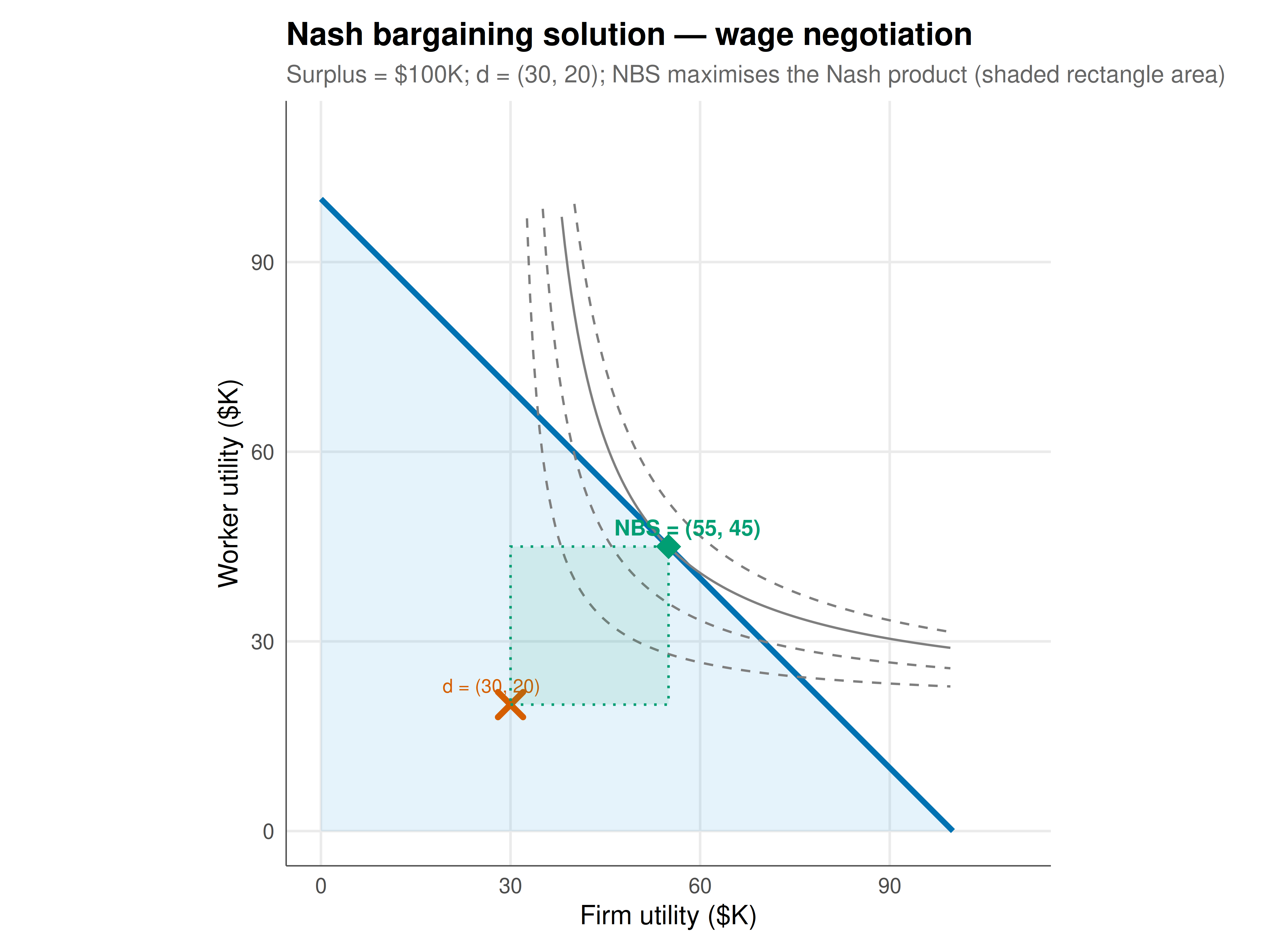
#| fig-cap: "Figure 1. Nash bargaining solution for a wage negotiation (linear Pareto frontier). The feasible set is shaded blue; the disagreement point d = (30, 20) is marked with ×. The Nash bargaining solution (green diamond) maximises the Nash product — the area of the rectangle from d to the frontier. Dashed curves show level sets of the Nash product (u₁−d₁)(u₂−d₂) = c. The solution splits the surplus according to relative bargaining position. Okabe-Ito palette."
#| dev: [png, pdf]
#| fig-width: 8
#| fig-height: 6
#| dpi: 300
# Wage negotiation visualization
d <- c(30, 20)
u1_range <- seq(0, 100, by = 0.5)
frontier <- tibble(u1 = u1_range, u2 = 100 - u1)

# Nash product level curves
nbs <- result_wage
level_curves <- lapply(c(200, 400, nbs$nash_product, 800), function(c) {
  u1_lc <- seq(d[1] + 0.1, 100, by = 0.5)
  u2_lc <- c / (u1_lc - d[1]) + d[2]
  tibble(u1 = u1_lc, u2 = u2_lc, level = c) |>
    filter(u2 > 0, u2 < 100)
})
lc_df <- bind_rows(level_curves) |>
  mutate(is_optimal = abs(level - nbs$nash_product) < 1)

# Feasible set polygon
feasible <- tibble(u1 = c(0, 100, 0, 0), u2 = c(100, 0, 0, 100))

p_nbs <- ggplot() +
  geom_polygon(data = feasible, aes(x = u1, y = u2),
               fill = okabe_ito[2], alpha = 0.15) +
  geom_line(data = frontier |> filter(u1 >= 0, u2 >= 0),
            aes(x = u1, y = u2), color = okabe_ito[5], linewidth = 1.2) +
  geom_line(data = lc_df, aes(x = u1, y = u2, group = level, linetype = is_optimal),
            color = "grey50", linewidth = 0.5) +
  # Disagreement point
  geom_point(aes(x = d[1], y = d[2]), shape = 4, size = 4, stroke = 2, color = okabe_ito[6]) +
  annotate("text", x = d[1] - 3, y = d[2] + 3, label = "d = (30, 20)",
           size = 3, color = okabe_ito[6]) +
  # Nash bargaining solution
  geom_point(aes(x = nbs$u1, y = nbs$u2), shape = 18, size = 5, color = okabe_ito[3]) +
  annotate("text", x = nbs$u1 + 3, y = nbs$u2 + 3,
           label = sprintf("NBS = (%.0f, %.0f)", nbs$u1, nbs$u2),
           size = 3.5, color = okabe_ito[3], fontface = "bold") +
  # Rectangle showing Nash product
  geom_rect(aes(xmin = d[1], xmax = nbs$u1, ymin = d[2], ymax = nbs$u2),
            fill = okabe_ito[3], alpha = 0.1, color = okabe_ito[3], linetype = "dotted") +
  scale_linetype_manual(values = c("TRUE" = "solid", "FALSE" = "dashed"), guide = "none") +
  labs(
    title = "Nash bargaining solution — wage negotiation",
    subtitle = "Surplus = $100K; d = (30, 20); NBS maximises the Nash product (shaded rectangle area)",
    x = "Firm utility ($K)", y = "Worker utility ($K)"
  ) +
  coord_fixed(xlim = c(0, 110), ylim = c(0, 110)) +
  theme_publication()

p_nbs
```
## Interactive figure
```{r}
#| label: fig-nbs-interactive
# Sensitivity: how does the disagreement point affect the split?
d1_seq <- seq(0, 50, by = 2)
nbs_sensitivity <- tibble(d1 = d1_seq) |>
  rowwise() |>
  mutate(
    d2 = 20,
    nbs = list(nash_bargaining_linear(100, 1, d1, d2)),
    u1_star = nbs$u1,
    u2_star = nbs$u2,
    firm_share = u1_star / 100,
    text = paste0("d₁ = ", d1, "\nFirm gets: $", round(u1_star), "K",
                  "\nWorker gets: $", round(u2_star), "K")
  ) |>
  ungroup() |>
  select(-nbs)

p_sens <- ggplot(nbs_sensitivity) +
  geom_line(aes(x = d1, y = u1_star, color = "Firm", text = text), linewidth = 1) +
  geom_line(aes(x = d1, y = u2_star, color = "Worker", text = text), linewidth = 1) +
  geom_hline(yintercept = 50, linetype = "dashed", color = "grey60") +
  scale_color_manual(values = c(Firm = okabe_ito[5], Worker = okabe_ito[1]),
                      name = "Player") +
  labs(
    title = "How outside options affect the Nash bargaining split",
    subtitle = "Worker's outside option fixed at $20K; firm's varies. Better outside option → larger share.",
    x = "Firm's outside option ($K)", y = "Nash bargaining payoff ($K)"
  ) +
  theme_publication()

ggplotly(p_sens, tooltip = "text") |>
  config(displaylogo = FALSE,
         modeBarButtonsToRemove = c("select2d", "lasso2d"))
```
## Interpretation
The Nash bargaining solution provides a clean, axiomatically grounded answer to "who gets what" in cooperative settings. The key insight is that **outside options determine bargaining power**: in the wage negotiation, the firm's higher outside option ($30K vs $20K) translates to a larger share of the surplus ($55K vs $45K), even though the Pareto frontier is symmetric. The sensitivity analysis makes this vivid — as the firm's outside option improves, its Nash bargaining payoff increases linearly while the worker's decreases. This captures the real-world observation that parties with better alternatives extract more from negotiations. The Nash product geometry reveals why the solution is unique: the rectangular hyperbolas (level sets of the Nash product) are tangent to the Pareto frontier at exactly one point, and this tangency condition is equivalent to the axiomatic requirements. The Nash bargaining solution connects to many areas of game theory: it is the unique symmetric solution to the bargaining problem, it can be implemented via the Rubinstein alternating-offers model (in the limit of patient players), and it appears as the cooperative counterpart to non-cooperative equilibrium analysis. In applied work, it is used to model wage setting (labour economics), international treaty design, merger negotiations, and any bilateral negotiation with well-defined outside options.
## Extensions & related tutorials
- [Mixed-strategy Nash equilibrium in 2×2 games](../nash-equilibrium-mixed/) — non-cooperative equilibrium for comparison.
- [The ultimatum game](../../classical-games/ultimatum-game/) — non-cooperative bargaining with take-it-or-leave-it offers.
- [Rubinstein bargaining model](../../cooperative-gt/rubinstein-alternating-offers/) — strategic foundations of Nash bargaining.
- [World Bank WDI indicators](../../public-apis-and-datasets/world-bank-wdi-economic-indicators/) — calibrating outside options with real data.
- [Cuban Missile Crisis](../../real-world-data-applications/cuban-missile-crisis-signaling-game/) — bargaining under nuclear threat.
## References
::: {#refs}
:::