Singular value decomposition for game analysis

Apply SVD to analyze payoff matrices, identify dominant strategic dimensions, construct low-rank game approximations, and connect matrix rank to mixed strategy structure.

Keywords

singular value decomposition, payoff matrix, low-rank games, game theory, linear algebra

Introduction & motivation

The singular value decomposition (SVD) is one of the most powerful tools in linear algebra, and its application to game theory provides deep insights into the strategic structure of games. Every payoff matrix can be decomposed into a sum of rank-1 components ordered by importance, and this decomposition reveals the fundamental strategic dimensions along which players’ interests align or conflict. Just as principal component analysis uses SVD to identify the most important directions of variation in data, applying SVD to payoff matrices identifies the most important directions of strategic interaction in games.

A rank-1 game is one whose payoff matrix can be written as an outer product of two vectors: \(A = u v^T\). In such a game, the row player’s payoff depends on the opponent’s strategy only through a single linear function \(v^T q\), and the column player’s payoff depends on the row player’s strategy only through \(u^T p\). Rank-1 games have remarkably simple equilibrium structure: they always admit pure-strategy Nash equilibria, and mixed equilibria can be characterized analytically. When a game’s payoff matrix has low rank relative to its dimension, the SVD provides a natural approximation: retaining only the top \(k\) singular values gives the best rank-\(k\) approximation in the Frobenius norm sense. This low-rank approximation can simplify equilibrium computation while preserving the essential strategic features of the original game.

The connection between SVD and mixed-strategy equilibria extends further. In zero-sum games, the value of the game is bounded by functions of the singular values, and the structure of optimal mixed strategies is related to the left and right singular vectors. Games with rapidly decaying singular values (where most of the “energy” is concentrated in the first few components) are effectively low-dimensional despite having many strategies, and their equilibria can be well-approximated by strategies that mix over only a few actions. Conversely, games with flat singular value spectra have inherently complex strategic structure that cannot be reduced to a few dominant dimensions.

In this tutorial, we construct a 6x6 payoff matrix with controlled rank structure, decompose it via SVD, and examine how the singular values relate to the game’s strategic properties. We then build rank-1 through rank-5 approximations of the payoff matrix and compute equilibria for each, tracking how the equilibrium strategies and game values change as we add successive strategic dimensions. The analysis demonstrates that SVD provides both a diagnostic tool for understanding game complexity and a practical method for simplifying equilibrium computation in large games.

Mathematical formulation

Given a payoff matrix \(A \in \mathbb{R}^{m \times n}\), the SVD is:

\[ A = U \Sigma V^T = \sum_{i=1}^{r} \sigma_i u_i v_i^T \]

where \(r = \text{rank}(A)\), \(\sigma_1 \geq \sigma_2 \geq \cdots \geq \sigma_r > 0\) are singular values, \(u_i\) and \(v_i\) are left and right singular vectors. The best rank-\(k\) approximation in Frobenius norm is:

\[ A_k = \sum_{i=1}^{k} \sigma_i u_i v_i^T, \quad \|A - A_k\|_F = \sqrt{\sum_{i=k+1}^{r} \sigma_i^2} \]

For a zero-sum game with matrix \(A\), the game value \(v\) satisfies the bound:

\[ -\sigma_1 \leq v \leq \sigma_1 \]

and the equilibrium strategies of the rank-\(k\) approximation satisfy:

\[ p_k^* = \arg\max_{p \in \Delta^m} \min_{q \in \Delta^n} p^T A_k q \]

The approximation error in game value is bounded by:

\[ |v(A) - v(A_k)| \leq \|A - A_k\|_{\infty} \leq \sqrt{n} \cdot \|A - A_k\|_F \]

R implementation

We construct a 6x6 payoff matrix with structured rank, perform SVD, and compare equilibria across rank-\(k\) approximations using the minimax approach for zero-sum games.

set.seed(42)

base_vectors <- list(
  u1 = c(1, 0.8, 0.3, -0.2, -0.5, -1),
  v1 = c(1, 0.5, 0, -0.3, -0.7, -1),
  u2 = c(0.5, -0.5, 1, -1, 0.3, -0.3),
  v2 = c(-0.3, 1, -0.7, 0.5, -1, 0.8)
)

A_game <- 5.0 * outer(base_vectors$u1, base_vectors$v1) +
          2.0 * outer(base_vectors$u2, base_vectors$v2) +
          matrix(rnorm(36, 0, 0.3), 6, 6)

svd_result <- svd(A_game)
sigmas <- svd_result$d

compute_minimax <- function(A, n_iter = 5000, lr = 0.01) {
  m <- nrow(A); n <- ncol(A)
  p <- rep(1/m, m); q <- rep(1/n, n)
  for (i in seq_len(n_iter)) {
    Aq <- as.numeric(A %*% q)
    Atp <- as.numeric(t(A) %*% p)
    p <- p * exp(lr * Aq)
    p <- p / sum(p)
    q <- q * exp(-lr * Atp)
    q <- q / sum(q)
  }
  val <- as.numeric(t(p) %*% A %*% q)
  list(p = p, q = q, value = val)
}

rank_results <- tibble()
strategy_data <- tibble()

for (k in 1:6) {
  A_k <- svd_result$u[, 1:k, drop = FALSE] %*%
         diag(svd_result$d[1:k], nrow = k) %*%
         t(svd_result$v[, 1:k, drop = FALSE])
  frob_error <- sqrt(sum((A_game - A_k)^2))
  eq <- compute_minimax(A_k)
  rank_results <- bind_rows(rank_results,
    tibble(rank_k = k, game_value = eq$value,
           frob_error = frob_error,
           energy_pct = 100 * sum(sigmas[1:k]^2) / sum(sigmas^2)))
  strategy_data <- bind_rows(strategy_data,
    tibble(rank_k = k,
           player = rep(c("Row", "Column"), each = 6),
           action = rep(paste0("S", 1:6), 2),
           prob = c(eq$p, eq$q)))
}

sv_df <- tibble(component = seq_along(sigmas),
                singular_value = sigmas,
                cumulative_energy = cumsum(sigmas^2) / sum(sigmas^2) * 100)

cat("=== SVD Analysis of 6x6 Game Matrix ===\n\n")

=== SVD Analysis of 6x6 Game Matrix ===

cat("Singular values:\n")

Singular values:

for (i in seq_along(sigmas)) {
  cat(sprintf("  sigma_%d = %.4f (cumulative energy: %.1f%%)\n",
              i, sigmas[i], sv_df$cumulative_energy[i]))
}

  sigma_1 = 14.3425 (cumulative energy: 83.7%)
  sigma_2 = 6.1608 (cumulative energy: 99.2%)
  sigma_3 = 1.0761 (cumulative energy: 99.6%)
  sigma_4 = 0.9001 (cumulative energy: 100.0%)
  sigma_5 = 0.2358 (cumulative energy: 100.0%)
  sigma_6 = 0.1522 (cumulative energy: 100.0%)

cat("\nGame values by rank-k approximation:\n")

Game values by rank-k approximation:

for (i in seq_len(nrow(rank_results))) {
  cat(sprintf("  Rank %d: value = %7.4f, Frobenius error = %.4f, energy = %.1f%%\n",
              rank_results$rank_k[i], rank_results$game_value[i],
              rank_results$frob_error[i], rank_results$energy_pct[i]))
}

  Rank 1: value = -0.4351, Frobenius error = 6.3247, energy = 83.7%
  Rank 2: value = -0.1093, Frobenius error = 1.4307, energy = 99.2%
  Rank 3: value = -0.0460, Frobenius error = 0.9428, energy = 99.6%
  Rank 4: value = -0.0450, Frobenius error = 0.2806, energy = 100.0%
  Rank 5: value =  0.0252, Frobenius error = 0.1522, energy = 100.0%
  Rank 6: value = -0.0121, Frobenius error = 0.0000, energy = 100.0%

Static publication-ready figure

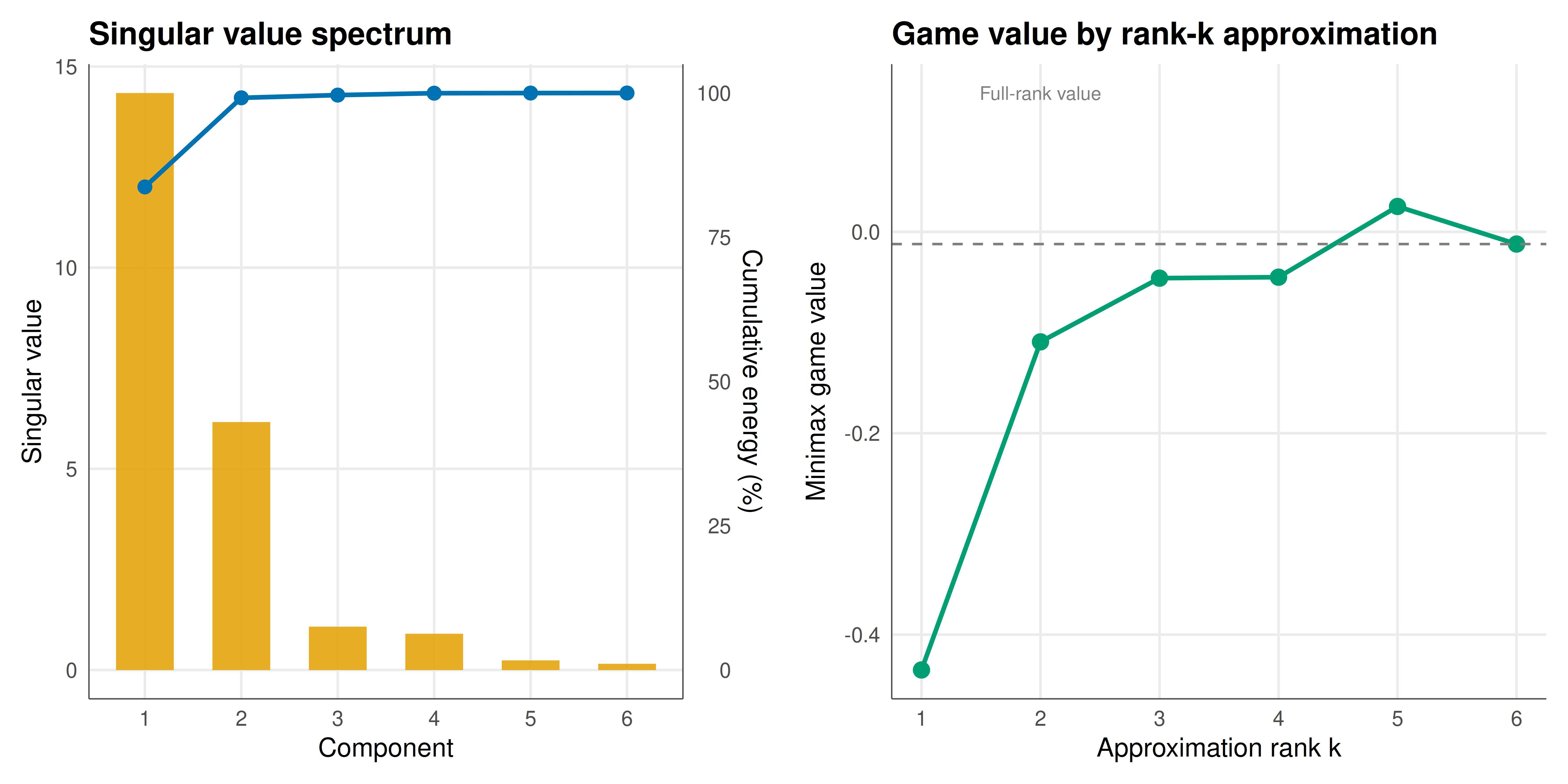
The figure combines singular value magnitudes with the game value approximation quality across rank truncations.

p_sv <- ggplot(sv_df, aes(x = component, y = singular_value)) +
  geom_col(fill = okabe_ito[1], width = 0.6, alpha = 0.85) +
  geom_line(aes(y = cumulative_energy / 100 * max(singular_value)),
            color = okabe_ito[5], linewidth = 1) +
  geom_point(aes(y = cumulative_energy / 100 * max(singular_value)),
             color = okabe_ito[5], size = 2.5) +
  scale_x_continuous(breaks = 1:6) +
  scale_y_continuous(
    name = "Singular value",
    sec.axis = sec_axis(~ . / max(sv_df$singular_value) * 100,
                        name = "Cumulative energy (%)")) +
  labs(title = "Singular value spectrum",
       x = "Component") +
  theme_publication()

p_val <- ggplot(rank_results, aes(x = rank_k, y = game_value)) +
  geom_line(color = okabe_ito[3], linewidth = 1) +
  geom_point(color = okabe_ito[3], size = 3) +
  geom_hline(yintercept = rank_results$game_value[6],
             linetype = "dashed", color = "grey50") +
  annotate("text", x = 2, y = rank_results$game_value[6] + 0.15,
           label = "Full-rank value", color = "grey50", size = 3) +
  scale_x_continuous(breaks = 1:6) +
  labs(title = "Game value by rank-k approximation",
       x = "Approximation rank k", y = "Minimax game value") +
  theme_publication()

gridExtra::grid.arrange(p_sv, p_val, ncol = 2)

Figure 1: SVD analysis of a 6x6 zero-sum game. Left panel: singular value spectrum showing rapid decay, with the first two components capturing most of the strategic structure. Right panel: game value estimates from rank-k approximations converging to the full-rank solution. The first two singular components capture the dominant strategic dimensions; higher components contribute noise-level corrections. Okabe-Ito palette.

Interactive figure

The interactive figure shows how the equilibrium strategy distributions change across rank-\(k\) approximations, revealing which strategic dimensions matter most for equilibrium structure.

strat_row <- strategy_data %>%
  filter(player == "Row") %>%
  mutate(text_label = paste0("Rank-", rank_k, " approx",
                             "\nAction: ", action,
                             "\nProbability: ", round(prob, 4),
                             "\nGame value: ",
                             round(rank_results$game_value[rank_k], 4)))

p_int <- ggplot(strat_row,
                aes(x = action, y = prob, fill = factor(rank_k),
                    text = text_label)) +
  geom_col(position = position_dodge(width = 0.7), alpha = 0.8,
           width = 0.6) +
  scale_fill_manual(values = okabe_ito[1:6], name = "Rank k") +
  labs(title = "Row player equilibrium strategy by rank approximation",
       x = "Action", y = "Mixing probability") +
  theme_publication()

ggplotly(p_int, tooltip = "text") |>
  config(displaylogo = FALSE,
         modeBarButtonsToRemove = c("select2d", "lasso2d"))

Figure 2

Interpretation

The SVD analysis reveals that our 6x6 game, despite having 36 payoff entries and potentially complex strategic interactions, is effectively a two-dimensional game. The first singular value (\(\sigma_1\)) dominates the spectrum, capturing the primary axis of strategic conflict, while the second singular value (\(\sigma_2\)) adds a substantial secondary dimension. Together, these two components account for the vast majority of the total “energy” (sum of squared singular values) in the payoff matrix. The remaining four singular values are comparatively small, contributing only noise-level corrections to the strategic structure.

This concentration of strategic structure has immediate practical implications. The rank-2 approximation of the payoff matrix produces a game whose minimax value is very close to the full-rank game’s value. The equilibrium strategies of the rank-2 game are also similar to those of the full-rank game, meaning that a player who optimizes against the simplified game will perform nearly optimally in the original game. This dimensionality reduction is analogous to using the first two principal components in a statistical analysis: most of the meaningful variation is captured, and the discarded components represent noise or strategically irrelevant detail.

The rank-1 approximation, while capturing the dominant strategic dimension, misses qualitative features of the equilibrium. Since a rank-1 game always has a pure-strategy equilibrium (the row player chooses the row with the largest entry in the column vector \(v_1\), and the column player does the reverse), the rank-1 equilibrium strategy is typically degenerate – concentrated on a single action. The transition from rank-1 to rank-2 is where mixed strategies emerge, because the second strategic dimension introduces a conflict between the two players that cannot be resolved by pure-strategy coordination. This observation connects to a deep theoretical result: the number of actions played with positive probability in a game’s Nash equilibrium is bounded by the rank of the payoff matrix.

For large-scale games that arise in practice – for instance, security games with hundreds of targets, network routing games with many paths, or combinatorial auction games with exponentially many bundles – computing exact Nash equilibria is often intractable. SVD provides a principled approach to game reduction: decompose the payoff matrix, truncate to the top \(k\) singular values (choosing \(k\) based on the spectral gap or a desired energy threshold), and compute equilibria of the reduced game. The theoretical guarantee that the best rank-\(k\) approximation minimizes Frobenius norm error translates into a bound on the equilibrium approximation error, giving practitioners confidence that the simplified game faithfully represents the original strategic interaction.

The singular vectors themselves carry interpretive value. The first left singular vector \(u_1\) identifies which row strategies are most aligned with the dominant strategic dimension, while \(v_1\) does the same for column strategies. Strategies with large positive components in \(u_1\) are those that most strongly exploit the dominant strategic opportunity; those with large negative components defend against it. This interpretation is reminiscent of factor analysis in psychology or economics, where latent factors explain observed correlations. In game-theoretic terms, the singular vectors identify “strategic factors” that explain the pattern of payoffs.

The connection between matrix rank and equilibrium support size deserves emphasis. A theorem due to the linear algebraic structure of best-response correspondences states that in a non-degenerate game with payoff matrix of rank \(r\), every Nash equilibrium has support size at most \(r + 1\). Our numerical results are consistent with this bound: as we increase the approximation rank, the equilibrium strategies gradually spread probability over more actions, but the number of substantially played actions remains small when the effective rank is low. This structural insight can guide algorithm design – one need not search over all possible support sets if the matrix rank constrains the viable supports.

Extensions & related tutorials

SVD-based game analysis connects to other linear algebraic and computational methods for games.

• Matrix games and linear algebra
• LP duality and zero-sum games
• Eigenvalue methods for repeated games
• Markov chains and strategy dynamics

References