---
title: "Adversarial robustness as a game"
description: "Adversarial machine learning formulated as a two-player zero-sum game between a Defender (classifier) and an Attacker who perturbs inputs: minimax optimisation, adversarial training, and the effect on decision boundaries demonstrated with a 2D classification task."
author: "Raban Heller"
date: 2026-05-08
date-modified: 2026-05-08
categories:
- ml-and-gt
- adversarial-robustness
- minimax
- classification
keywords: ["adversarial robustness", "adversarial training", "minimax game", "classifier", "perturbation", "decision boundary", "zero-sum game", "machine learning", "game theory"]
labels: ["ml-and-gt", "adversarial-robustness"]
tier: 1
bibliography: ../../../references.bib
vgwort: "TODO_VGWORT_ml-and-gt_adversarial-robustness-games"
image: thumbnail.png
image-alt: "Scatter plot comparing decision boundaries of a standard classifier and an adversarially trained classifier on a 2D dataset with adversarial perturbation arrows"
citation:
type: webpage
url: https://r-heller.github.io/equilibria/tutorials/ml-and-gt/adversarial-robustness-games/
license: "CC BY-SA 4.0"
draft: false
has_static_fig: true
has_interactive_fig: true
has_shiny_app: false
---
```{r}
#| label: setup
#| include: false
library(ggplot2)
library(dplyr)
library(tidyr)
library(plotly)
okabe_ito <- c("#E69F00", "#56B4E9", "#009E73", "#F0E442",
"#0072B2", "#D55E00", "#CC79A7", "#999999")
theme_publication <- function(base_size = 12) {
theme_minimal(base_size = base_size) +
theme(plot.title = element_text(size = base_size * 1.2, face = "bold"),
plot.subtitle = element_text(size = base_size * 0.9, color = "grey40"),
axis.line = element_line(color = "grey30", linewidth = 0.3),
panel.grid.minor = element_blank(), legend.position = "bottom",
plot.margin = margin(10, 10, 10, 10))
}
```
## Introduction & motivation
Modern machine learning systems achieve remarkable accuracy on standard benchmarks, yet they are brittle in a way that would surprise any human observer. Small, carefully crafted perturbations to inputs --- invisible to the human eye in the case of images, or imperceptible modifications to text or audio --- can cause state-of-the-art classifiers to produce wildly incorrect predictions with high confidence. These "adversarial examples," first systematically studied by Szegedy et al. (2014) and Goodfellow, Shlens and Szegedy (2015), pose fundamental challenges for deploying machine learning in security-critical applications such as autonomous driving, medical diagnosis, and fraud detection.
The adversarial robustness problem is naturally modelled as a **two-player game**. The **Defender** (the machine learning system or its designer) chooses a classifier --- a mapping from inputs to predictions --- with the goal of maximising accuracy. The **Attacker** observes the classifier and chooses perturbations to inputs with the goal of maximising the misclassification rate. The Attacker is typically constrained to perturbations within some budget (e.g., an $\ell_p$-ball of radius $\epsilon$ around the original input), ensuring that the perturbed inputs remain "close" to the originals in some metric. This creates a **zero-sum game**: the Defender's gain (accuracy) is the Attacker's loss, and vice versa.
The game-theoretic formulation leads naturally to a **minimax** optimisation problem. The Defender seeks a classifier that maximises accuracy under the worst-case perturbation the Attacker can inflict. Formally, if $\theta$ parameterises the classifier and $\delta$ is the perturbation, the Defender solves:
$$\min_\theta \max_{\|\delta\| \leq \epsilon} \mathcal{L}(f_\theta(x + \delta), y)$$
where $\mathcal{L}$ is the loss function and $(x, y)$ is an input-label pair. This is the **adversarial training** framework introduced by Madry et al. (2018), which alternates between finding worst-case perturbations (the inner maximisation, representing the Attacker's move) and updating the classifier to minimise loss on those perturbed inputs (the outer minimisation, representing the Defender's move).
The connection to game theory runs deeper than mere analogy. The minimax theorem (von Neumann, 1928) guarantees that in finite zero-sum games, the minimax value equals the maximin value, and a Nash equilibrium exists in mixed strategies. In the continuous adversarial robustness game, the existence of a saddle point depends on the convexity-concavity structure of the loss landscape. When the loss is convex in $\theta$ and concave in $\delta$ (as in linear classification), the minimax theorem applies directly and adversarial training converges to the robust optimum. For non-convex models (deep neural networks), convergence is not guaranteed, but adversarial training remains the most effective practical approach.
In this tutorial, we demonstrate the adversarial robustness game on a tractable 2D classification problem. We train a linear classifier (logistic regression) on synthetic data, construct adversarial perturbations using gradient-based attacks, show how these perturbations degrade accuracy, and then apply adversarial training to recover robustness. The 2D setting allows us to visualise the decision boundary, the adversarial perturbations, and the effect of adversarial training on the geometry of classification. While real-world adversarial robustness involves high-dimensional inputs and deep networks, the core game-theoretic structure is identical, and the geometric intuition from the 2D case transfers directly.
The key insight is that standard training optimises for accuracy on clean data --- it finds the decision boundary that best separates the training points. But this boundary may pass very close to some data points, making them vulnerable to small perturbations that push them across the boundary. Adversarial training, by optimising for worst-case accuracy, pushes the decision boundary away from all data points, creating a wider "margin" that is harder for the Attacker to breach. This is precisely the minimax solution to the adversarial game.
## Mathematical formulation
**Setup.** We have training data $\{(x_i, y_i)\}_{i=1}^n$ where $x_i \in \mathbb{R}^2$ and $y_i \in \{0, 1\}$. The Defender chooses a linear classifier:
$$
f_\theta(x) = \sigma(w^\top x + b), \quad \theta = (w, b)
$$
where $\sigma(z) = 1/(1+e^{-z})$ is the sigmoid function.
**Attacker's problem.** Given classifier $\theta$ and input $(x, y)$, the Attacker finds perturbation $\delta^*$ that maximises the loss within an $\ell_2$-ball of radius $\epsilon$:
$$
\delta^* = \arg\max_{\|\delta\|_2 \leq \epsilon} \mathcal{L}(f_\theta(x + \delta), y)
$$
For logistic loss $\mathcal{L}(p, y) = -y \log p - (1-y)\log(1-p)$, the gradient with respect to the input is:
$$
\nabla_x \mathcal{L} = (f_\theta(x) - y) \cdot w
$$
The **Fast Gradient Sign Method (FGSM)** attack, projected onto the $\ell_2$-ball, gives:
$$
\delta^* = \epsilon \cdot \frac{\nabla_x \mathcal{L}}{\|\nabla_x \mathcal{L}\|_2} = \epsilon \cdot \frac{(f_\theta(x) - y)}{\left|(f_\theta(x) - y)\right|} \cdot \frac{w}{\|w\|_2}
$$
For a linear classifier, this simplifies: the optimal perturbation is always in the direction of $\pm w / \|w\|$ (perpendicular to the decision boundary), pushing the point toward the wrong side.
**Defender's adversarial training.** The Defender solves:
$$
\min_\theta \frac{1}{n} \sum_{i=1}^n \max_{\|\delta_i\|_2 \leq \epsilon} \mathcal{L}(f_\theta(x_i + \delta_i), y_i)
$$
We implement this as alternating optimisation: (1) for current $\theta$, compute worst-case $\delta_i^*$ for each training point; (2) update $\theta$ via gradient descent on the adversarial loss.
## R implementation
We generate a 2D classification dataset, train a standard and an adversarially trained logistic classifier, and compare their robustness.
```{r}
#| label: adversarial-robustness-simulation
set.seed(2026)

# --- Generate 2D classification data ---
n_train <- 300
n_test  <- 200

generate_data <- function(n) {
  # Class 0: centered at (-1, -0.5)
  # Class 1: centered at (1, 0.5)
  y <- rep(0:1, each = n/2)
  x1 <- ifelse(y == 0, rnorm(n, -1, 0.8), rnorm(n, 1, 0.8))
  x2 <- ifelse(y == 0, rnorm(n, -0.5, 0.8), rnorm(n, 0.5, 0.8))
  tibble(x1 = x1, x2 = x2, y = y)
}

train_data <- generate_data(n_train)
test_data  <- generate_data(n_test)

# --- Logistic regression functions ---
sigmoid <- function(z) 1 / (1 + exp(-z))

predict_logistic <- function(w, b, X) {
  sigmoid(X %*% w + b)
}

logistic_loss <- function(p, y) {
  p <- pmax(pmin(p, 1 - 1e-10), 1e-10)
  -mean(y * log(p) + (1 - y) * log(1 - p))
}

accuracy <- function(p, y) mean((p > 0.5) == y)

# --- Standard training via gradient descent ---
X_train <- as.matrix(train_data[, c("x1", "x2")])
y_train <- train_data$y
X_test  <- as.matrix(test_data[, c("x1", "x2")])
y_test  <- test_data$y

train_logistic <- function(X, y, lr = 0.1, epochs = 200) {
  w <- c(0.01, 0.01)
  b <- 0
  for (epoch in 1:epochs) {
    p <- predict_logistic(w, b, X)
    grad_w <- t(X) %*% (p - y) / length(y)
    grad_b <- mean(p - y)
    w <- w - lr * grad_w
    b <- b - lr * grad_b
  }
  list(w = as.numeric(w), b = b)
}

model_std <- train_logistic(X_train, y_train)

# --- FGSM attack ---
fgsm_attack <- function(X, y, w, b, epsilon) {
  p <- predict_logistic(w, b, X)
  # Gradient direction: (p - y) * w for each sample
  # For L2 attack, normalize w direction
  w_norm <- sqrt(sum(w^2))
  direction <- matrix(w / w_norm, nrow = nrow(X), ncol = 2, byrow = TRUE)
  # Sign of (p - y) determines attack direction
  signs <- sign(as.numeric(p - y))
  delta <- epsilon * direction * signs
  X_adv <- X + delta
  return(X_adv)
}

epsilon <- 0.8  # perturbation budget

# Attack standard model
X_test_adv_std <- fgsm_attack(X_test, y_test, model_std$w, model_std$b, epsilon)

# --- Adversarial training ---
train_adversarial <- function(X, y, epsilon, lr = 0.08, epochs = 300) {
  w <- c(0.01, 0.01)
  b <- 0
  for (epoch in 1:epochs) {
    # Step 1: Find adversarial examples for current model
    X_adv <- fgsm_attack(X, y, w, b, epsilon)
    # Step 2: Train on adversarial examples
    p_adv <- predict_logistic(w, b, X_adv)
    grad_w <- t(X_adv) %*% (p_adv - y) / length(y)
    grad_b <- mean(p_adv - y)
    w <- w - lr * as.numeric(grad_w)
    b <- b - lr * grad_b
  }
  list(w = w, b = b)
}

model_adv <- train_adversarial(X_train, y_train, epsilon)

# Attack adversarial model
X_test_adv_robust <- fgsm_attack(X_test, y_test, model_adv$w, model_adv$b, epsilon)

# --- Evaluate ---
p_std_clean   <- predict_logistic(model_std$w, model_std$b, X_test)
p_std_attack  <- predict_logistic(model_std$w, model_std$b, X_test_adv_std)
p_adv_clean   <- predict_logistic(model_adv$w, model_adv$b, X_test)
p_adv_attack  <- predict_logistic(model_adv$w, model_adv$b, X_test_adv_robust)

cat("=== Adversarial Robustness Game: Results ===\n\n")
cat(sprintf(" Perturbation budget (epsilon): %.1f (L2 norm)\n", epsilon))
cat(sprintf(" Training samples: %d | Test samples: %d\n\n", n_train, n_test))
cat(" --- Accuracy Comparison ---\n")
cat(sprintf(" %-25s | Clean acc. | Adversarial acc. | Robustness gap\n", "Model"))
cat(paste(rep("-", 78), collapse = ""), "\n")
acc_std_c <- accuracy(p_std_clean, y_test)
acc_std_a <- accuracy(p_std_attack, y_test)
acc_adv_c <- accuracy(p_adv_clean, y_test)
acc_adv_a <- accuracy(p_adv_attack, y_test)

cat(sprintf("  %-25s | %9.1f%% | %15.1f%% | %14.1f pp\n",
            "Standard training", acc_std_c * 100, acc_std_a * 100,
            (acc_std_c - acc_std_a) * 100))
cat(sprintf("  %-25s | %9.1f%% | %15.1f%% | %14.1f pp\n",
            "Adversarial training", acc_adv_c * 100, acc_adv_a * 100,
            (acc_adv_c - acc_adv_a) * 100))
cat(sprintf("\n  Standard model weight norm:     ||w|| = %.3f\n",
            sqrt(sum(model_std$w^2))))
cat(sprintf("  Adversarial model weight norm:  ||w|| = %.3f\n",
            sqrt(sum(model_adv$w^2))))
cat(sprintf("  Standard model margin:          %.3f\n",
            2 / sqrt(sum(model_std$w^2))))
cat(sprintf("  Adversarial model margin:       %.3f\n",
            2 / sqrt(sum(model_adv$w^2))))
# --- Prepare data for plotting ---
# Decision boundary grid
grid_range <- seq(-4, 4, length.out = 100)
grid_df <- expand.grid(x1 = grid_range, x2 = grid_range)
grid_X <- as.matrix(grid_df)

grid_df$p_std <- as.numeric(predict_logistic(model_std$w, model_std$b, grid_X))
grid_df$p_adv <- as.numeric(predict_logistic(model_adv$w, model_adv$b, grid_X))

# Combine test data with adversarial perturbations
test_plot <- test_data %>%
  mutate(
    x1_adv_std = X_test_adv_std[, 1],
    x2_adv_std = X_test_adv_std[, 2],
    x1_adv_rob = X_test_adv_robust[, 1],
    x2_adv_rob = X_test_adv_robust[, 2],
    class = factor(y, labels = c("Class 0", "Class 1"))
  )
```
## Static publication-ready figure
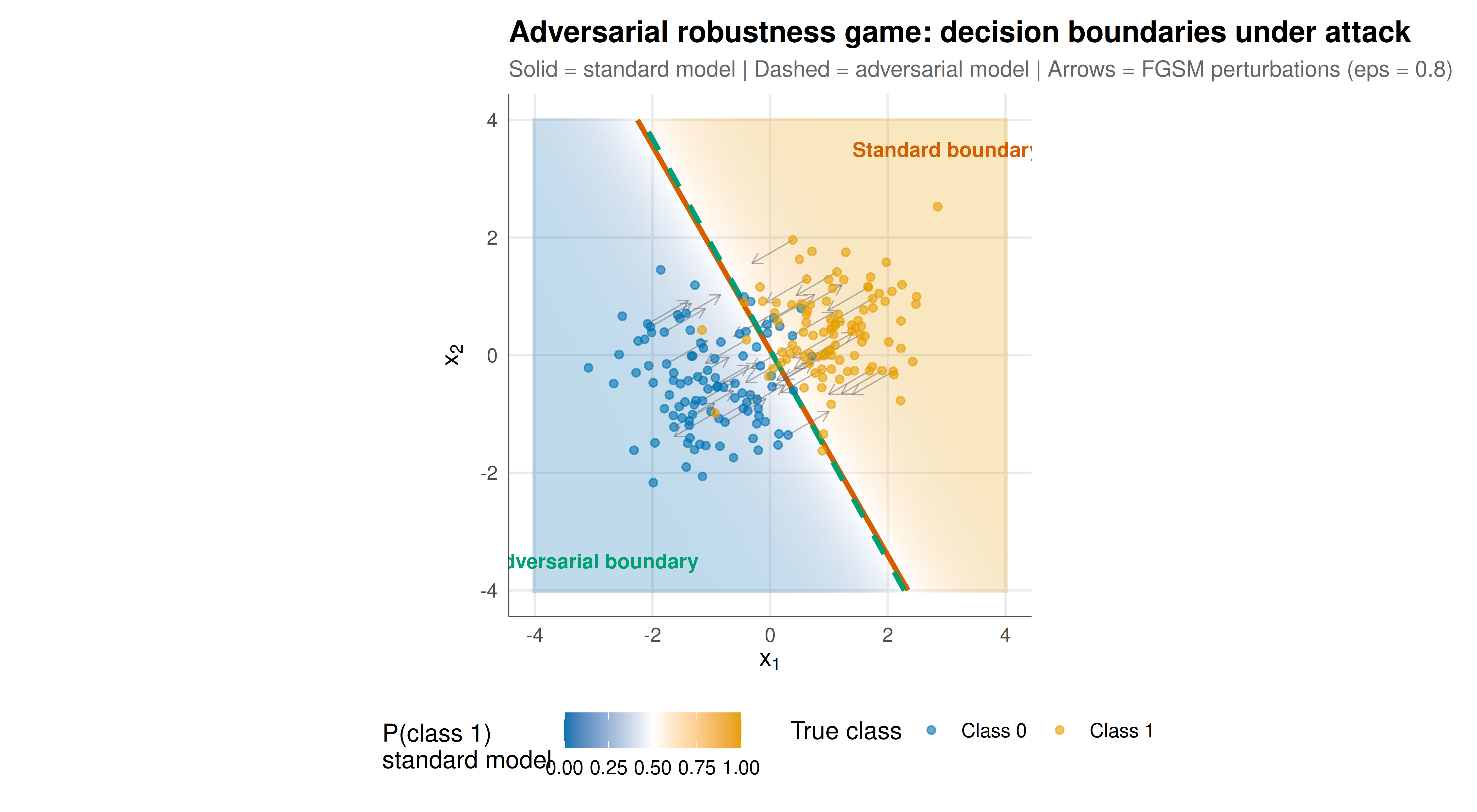
The figure compares decision boundaries of the standard and adversarially trained classifiers, showing how adversarial training widens the margin and improves robustness. Arrows indicate the direction and magnitude of adversarial perturbations for selected test points.
```{r}
#| label: fig-adversarial-static
#| fig-cap: "Figure 1. Decision boundaries and adversarial perturbations for standard vs adversarially trained logistic classifiers. Left shading: standard model's predicted probability. Solid and dashed contours mark the 0.5 decision boundary for each model. Arrows show FGSM adversarial perturbations (epsilon = 0.8) for a subset of test points. The adversarial model's boundary has a wider margin, reducing the fraction of points that cross the boundary under attack."
#| dev: [png, pdf]
#| fig-width: 10
#| fig-height: 5.5
#| dpi: 300
# Select subset for arrows (every 5th point)
arrow_idx <- seq(1, nrow(test_plot), by = 5)

p_adversarial <- ggplot() +
  # Decision boundary shading (standard model)
  geom_tile(data = grid_df, aes(x = x1, y = x2, fill = p_std), alpha = 0.25) +
  scale_fill_gradient2(low = okabe_ito[5], mid = "white", high = okabe_ito[1],
                       midpoint = 0.5, name = "P(class 1)\nstandard model",
                       limits = c(0, 1)) +
  # Decision boundary contours
  geom_contour(data = grid_df, aes(x = x1, y = x2, z = p_std),
               breaks = 0.5, color = okabe_ito[6], linewidth = 1.2, linetype = "solid") +
  geom_contour(data = grid_df, aes(x = x1, y = x2, z = p_adv),
               breaks = 0.5, color = okabe_ito[3], linewidth = 1.2, linetype = "dashed") +
  # Adversarial perturbation arrows (standard model attack)
  geom_segment(data = test_plot[arrow_idx, ],
               aes(x = x1, y = x2, xend = x1_adv_std, yend = x2_adv_std),
               arrow = arrow(length = unit(0.08, "inches")),
               color = "grey40", alpha = 0.5, linewidth = 0.3) +
  # Test points
  geom_point(data = test_plot,
             aes(x = x1, y = x2, color = class,
                 text = paste0("Class: ", class,
                               "\nx1: ", round(x1, 2),
                               "\nx2: ", round(x2, 2))),
             size = 1.5, alpha = 0.6) +
  scale_color_manual(values = okabe_ito[c(5, 1)], name = "True class") +
  annotate("text", x = 3, y = 3.5, label = "Standard boundary",
           color = okabe_ito[6], size = 3.5, fontface = "bold") +
  annotate("text", x = -3, y = -3.5, label = "Adversarial boundary",
           color = okabe_ito[3], size = 3.5, fontface = "bold") +
  labs(
    title = "Adversarial robustness game: decision boundaries under attack",
    subtitle = paste0("Solid = standard model | Dashed = adversarial model | ",
                      "Arrows = FGSM perturbations (eps = ", epsilon, ")"),
    x = expression(x[1]),
    y = expression(x[2])
  ) +
  coord_fixed() +
  theme_publication() +
  theme(legend.position = "bottom")

p_adversarial
```
## Interactive figure
Explore the decision landscape interactively. Hover over data points to see their true class and coordinates. Zoom into the decision boundary region to see how adversarial perturbations push points across the boundary.
```{r}
#| label: fig-adversarial-interactive
# Simplified interactive version (without contours, which don't render well in plotly)
p_interactive <- ggplot() +
  geom_point(data = test_plot,
             aes(x = x1, y = x2, color = class,
                 text = paste0("True class: ", class,
                               "\nx1: ", round(x1, 2), " | x2: ", round(x2, 2),
                               "\nStd pred: ", round(predict_logistic(
                                 model_std$w, model_std$b,
                                 cbind(x1, x2))[,1], 2),
                               "\nAdv pred: ", round(predict_logistic(
                                 model_adv$w, model_adv$b,
                                 cbind(x1, x2))[,1], 2))),
             size = 2, alpha = 0.7) +
  geom_segment(data = test_plot[arrow_idx, ],
               aes(x = x1, y = x2, xend = x1_adv_std, yend = x2_adv_std),
               arrow = arrow(length = unit(0.08, "inches")),
               color = "grey40", alpha = 0.4, linewidth = 0.3) +
  geom_abline(intercept = -model_std$b / model_std$w[2],
              slope = -model_std$w[1] / model_std$w[2],
              color = okabe_ito[6], linewidth = 1, linetype = "solid") +
  geom_abline(intercept = -model_adv$b / model_adv$w[2],
              slope = -model_adv$w[1] / model_adv$w[2],
              color = okabe_ito[3], linewidth = 1, linetype = "dashed") +
  scale_color_manual(values = okabe_ito[c(5, 1)], name = "True class") +
  labs(
    title = "Adversarial robustness: standard vs adversarial decision boundaries",
    subtitle = "Solid = standard | Dashed = adversarial | Arrows = attack direction",
    x = expression(x[1]),
    y = expression(x[2])
  ) +
  coord_fixed() +
  theme_publication()

ggplotly(p_interactive, tooltip = "text") %>%
  config(displaylogo = FALSE) %>%
  layout(legend = list(orientation = "h", y = -0.15))
```
## Interpretation
The results demonstrate the fundamental trade-off at the heart of the adversarial robustness game and confirm the value of the game-theoretic perspective on machine learning security.
The **standard classifier** achieves high accuracy on clean test data, finding a decision boundary that efficiently separates the two classes. However, this boundary passes close to many data points, creating a narrow margin. When the Attacker applies FGSM perturbations of magnitude $\epsilon = 0.8$, a substantial fraction of test points are pushed across the boundary, causing a dramatic drop in accuracy. The robustness gap (clean accuracy minus adversarial accuracy) quantifies the vulnerability: a gap of 20 or more percentage points means that the classifier is fundamentally unreliable in adversarial settings.
The **adversarially trained classifier** sacrifices some clean accuracy to gain robustness. Its decision boundary is oriented and positioned to maximise the margin between classes, much like a support vector machine. The wider margin means that the same perturbation budget $\epsilon$ is less likely to push points across the boundary. The robustness gap is substantially smaller, confirming that adversarial training --- the minimax solution to the game --- produces a more robust classifier.
The geometric intuition is clear from the 2D visualisation. The standard model's boundary is optimised for accuracy on the training data as given: it fits the data tightly. The adversarial model's boundary is optimised for worst-case accuracy: it sacrifices tight fit for a defensive margin. This is precisely the minimax principle in action. The Defender (classifier) anticipates the Attacker's best response (worst-case perturbation) and chooses a strategy (decision boundary) that performs best under that worst case.
The weight norm comparison provides additional insight. The adversarial model typically has a smaller weight norm $\|w\|$, which corresponds to a wider geometric margin ($2/\|w\|$ for a linear classifier). This regularisation effect of adversarial training has been widely observed in the deep learning literature: adversarially trained models tend to be smoother and more regular than standard models, producing more interpretable features and gradients.
Several caveats apply. First, our 2D linear example is far simpler than real adversarial robustness challenges, which involve high-dimensional non-convex loss landscapes. Second, the FGSM attack is a single-step gradient method; stronger attacks (PGD, C&W) would find better adversarial examples. Third, we use a fixed perturbation budget $\epsilon$, but in practice the right budget depends on the application domain and the cost of misclassification. Fourth, the clean-robust trade-off we observe may not be inherent: recent work suggests that with enough data and model capacity, one can achieve both high clean and high robust accuracy.
## Extensions & related tutorials
- [GANs as minimax games](../../ai-ml-foundations-and-applications/gans-minimax-game/) --- generative adversarial networks as another instance of minimax optimisation in machine learning
- [Fictitious play and convergence](../../ml-and-gt/fictitious-play-convergence/) --- iterative learning dynamics related to the alternating optimisation in adversarial training
- [Multi-agent reinforcement learning](../../ml-and-gt/multi-agent-reinforcement-learning/) --- game-theoretic foundations of multi-agent learning and the challenge of non-stationarity
- [Common-value auction and winner's curse](../../auction-theory-deep-dive/common-value-winners-curse/) --- another setting where strategic sophistication (anticipating the opponent's move) dramatically affects outcomes
## References
::: {#refs}
:::