Deep reinforcement learning for strategic games

Implement simple deep RL agents from scratch in R that learn game strategies through self-play, comparing learned policies with analytical Nash equilibria.

Keywords

deep reinforcement learning, Q-learning, self-play, Nash equilibrium, neural network

Introduction & motivation

Reinforcement learning (RL) has achieved remarkable success in strategic games, from TD-Gammon’s mastery of backgammon in the 1990s to AlphaGo’s victory over world champion Go players in 2016 and AlphaStar’s grandmaster-level StarCraft II play. These achievements rely on deep reinforcement learning: combining neural network function approximation with RL algorithms to learn policies in environments with enormous state spaces. While the headline results involve vast computational resources and sophisticated architectures, the core principles are accessible and can be demonstrated on simple matrix games where analytical Nash equilibria provide a ground truth for evaluation.

The connection between reinforcement learning and game theory runs deep. In single-agent RL, the agent interacts with a stationary environment, and standard convergence results guarantee that Q-learning finds optimal policies under mild conditions. In multi-agent settings, however, the environment is non-stationary because each agent’s optimal policy depends on what the other agents are doing. This creates a moving-target problem: as one agent improves its strategy, the other agent’s Q-values change, potentially destabilizing convergence. The question of whether independent RL agents converge to Nash equilibria in general games remains one of the central open problems at the intersection of machine learning and game theory.

Self-play – where an agent trains by playing against copies of itself – is the dominant paradigm for applying RL to games. In self-play, both players update their strategies simultaneously based on the outcomes of their interactions. For zero-sum games, self-play with certain RL algorithms provably converges to minimax equilibria, but for general-sum games the convergence landscape is more complex and may involve cycling, chaos, or convergence to non-Nash fixed points. Understanding these dynamics requires implementing the algorithms from scratch and observing their behavior on games with known solutions.

This tutorial implements a minimal deep Q-learning agent entirely from scratch in R, using only base matrix operations for the neural network forward and backward passes – no external deep learning packages are required. We train two such agents through self-play on a 3x3 general-sum matrix game (a variant of the Battle of the Sexes with a third strategy) and track how their learned mixed strategies evolve over training episodes. The analytical Nash equilibrium of the game serves as our benchmark. We observe how the agents’ strategy profiles oscillate around the equilibrium, sometimes approaching it closely but never fully converging, illustrating the fundamental challenges of multi-agent learning. The implementation provides a transparent view into the mechanics of deep RL for games, showing exactly how gradients flow through the network and how Q-value estimates translate into action probabilities.

Mathematical formulation

We define a simple feedforward neural network with one hidden layer. Given input state vector \(x \in \mathbb{R}^d\), the Q-value predictions are:

\[ Q(x; \theta) = W_2 \cdot \text{ReLU}(W_1 x + b_1) + b_2 \]

where \(\theta = \{W_1, b_1, W_2, b_2\}\) are learnable parameters. The loss function for a single transition is the squared temporal difference error:

\[ L(\theta) = \frac{1}{2}\left(r + \gamma \max_{a'} Q(x'; \theta^{-}) - Q(x, a; \theta)\right)^2 \]

where \(r\) is the reward, \(\gamma\) is the discount factor, and \(\theta^{-}\) are target network parameters. The agent selects actions using an epsilon-greedy policy derived from a softmax over Q-values:

\[ \pi(a|x) = (1 - \varepsilon) \cdot \frac{\exp(Q(x,a) / \tau)}{\sum_{a'} \exp(Q(x,a') / \tau)} + \frac{\varepsilon}{|A|} \]

At a Nash equilibrium \((p^*, q^*)\) of the stage game, neither player can improve their expected payoff by unilateral deviation: \(p^{*T} A q^* \geq e_i^T A q^*\) for all pure strategies \(e_i\).

R implementation

We implement a neural network from scratch using matrix operations, then train two agents through self-play on a 3x3 game.

set.seed(42)

relu <- function(x) pmax(x, 0)
relu_grad <- function(x) ifelse(x > 0, 1, 0)

init_network <- function(input_dim, hidden_dim, output_dim) {
  list(
    W1 = matrix(rnorm(hidden_dim * input_dim, sd = 0.3),
                hidden_dim, input_dim),
    b1 = rep(0, hidden_dim),
    W2 = matrix(rnorm(output_dim * hidden_dim, sd = 0.3),
                output_dim, hidden_dim),
    b2 = rep(0, output_dim)
  )
}

forward <- function(net, x) {
  z1 <- net$W1 %*% x + net$b1
  a1 <- relu(z1)
  q <- net$W2 %*% a1 + net$b2
  list(q = as.numeric(q), z1 = z1, a1 = a1)
}

backward <- function(net, x, fwd, target_q, action, lr = 0.005) {
  dq <- rep(0, length(fwd$q))
  dq[action] <- fwd$q[action] - target_q
  dW2 <- matrix(dq, ncol = 1) %*% t(fwd$a1)
  db2 <- dq
  da1 <- t(net$W2) %*% dq
  dz1 <- da1 * relu_grad(fwd$z1)
  dW1 <- matrix(dz1, ncol = 1) %*% t(x)
  db1 <- as.numeric(dz1)
  net$W2 <- net$W2 - lr * dW2
  net$b2 <- net$b2 - lr * db2
  net$W1 <- net$W1 - lr * dW1
  net$b1 <- net$b1 - lr * db1
  net
}

softmax_policy <- function(q_vals, tau = 0.5, epsilon = 0.05) {
  exp_q <- exp((q_vals - max(q_vals)) / tau)
  probs <- (1 - epsilon) * exp_q / sum(exp_q) + epsilon / length(q_vals)
  probs / sum(probs)
}

A_pay <- matrix(c(3, 0, 1,
                   0, 2, 1,
                   1, 1, 1.5), nrow = 3, byrow = TRUE)
B_pay <- matrix(c(2, 0, 1,
                   0, 3, 1,
                   1, 1, 1.5), nrow = 3, byrow = TRUE)

n_actions <- 3
state <- matrix(c(1, 0, 0), ncol = 1)

net1 <- init_network(3, 16, n_actions)
net2 <- init_network(3, 16, n_actions)

n_episodes <- 2000
record_interval <- 20
strategy_history <- tibble()

for (ep in seq_len(n_episodes)) {
  fwd1 <- forward(net1, state)
  fwd2 <- forward(net2, state)
  pol1 <- softmax_policy(fwd1$q, tau = max(0.3, 1.0 - ep / 2000))
  pol2 <- softmax_policy(fwd2$q, tau = max(0.3, 1.0 - ep / 2000))
  a1 <- sample(seq_len(n_actions), 1, prob = pol1)
  a2 <- sample(seq_len(n_actions), 1, prob = pol2)
  r1 <- A_pay[a1, a2]
  r2 <- B_pay[a1, a2]
  target1 <- r1
  target2 <- r2
  net1 <- backward(net1, state, fwd1, target1, a1, lr = 0.003)
  net2 <- backward(net2, state, fwd2, target2, a2, lr = 0.003)

  if (ep %% record_interval == 0) {
    cur_fwd1 <- forward(net1, state)
    cur_fwd2 <- forward(net2, state)
    p1 <- softmax_policy(cur_fwd1$q, tau = 0.5, epsilon = 0)
    p2 <- softmax_policy(cur_fwd2$q, tau = 0.5, epsilon = 0)
    strategy_history <- bind_rows(strategy_history,
      tibble(episode = ep,
             player = rep(c("Player 1", "Player 2"), each = 3),
             action = rep(paste0("A", 1:3), 2),
             prob = c(p1, p2)))
  }
}

final_fwd1 <- forward(net1, state)
final_fwd2 <- forward(net2, state)
final_p1 <- softmax_policy(final_fwd1$q, tau = 0.5, epsilon = 0)
final_p2 <- softmax_policy(final_fwd2$q, tau = 0.5, epsilon = 0)

cat("=== Deep RL Self-Play Results ===\n\n")

=== Deep RL Self-Play Results ===

cat("Payoff matrix A (row player):\n")

Payoff matrix A (row player):

for (i in 1:3) cat(sprintf("  [%s]\n", paste(A_pay[i,], collapse = ", ")))

  [3, 0, 1]
  [0, 2, 1]
  [1, 1, 1.5]

cat("\nPayoff matrix B (column player):\n")

Payoff matrix B (column player):

for (i in 1:3) cat(sprintf("  [%s]\n", paste(B_pay[i,], collapse = ", ")))

  [2, 0, 1]
  [0, 3, 1]
  [1, 1, 1.5]

cat(sprintf("\nLearned Player 1 strategy: [%s]\n",
            paste(round(final_p1, 4), collapse = ", ")))

Learned Player 1 strategy: [0.9633, 0.0061, 0.0306]

cat(sprintf("Learned Player 2 strategy: [%s]\n",
            paste(round(final_p2, 4), collapse = ", ")))

Learned Player 2 strategy: [0.8454, 0.0184, 0.1362]

cat(sprintf("\nExpected payoff P1: %.4f\n",
            t(final_p1) %*% A_pay %*% final_p2))

Expected payoff P1: 2.6082

cat(sprintf("Expected payoff P2: %.4f\n",
            t(final_p1) %*% B_pay %*% final_p2))

Expected payoff P2: 1.7939

Static publication-ready figure

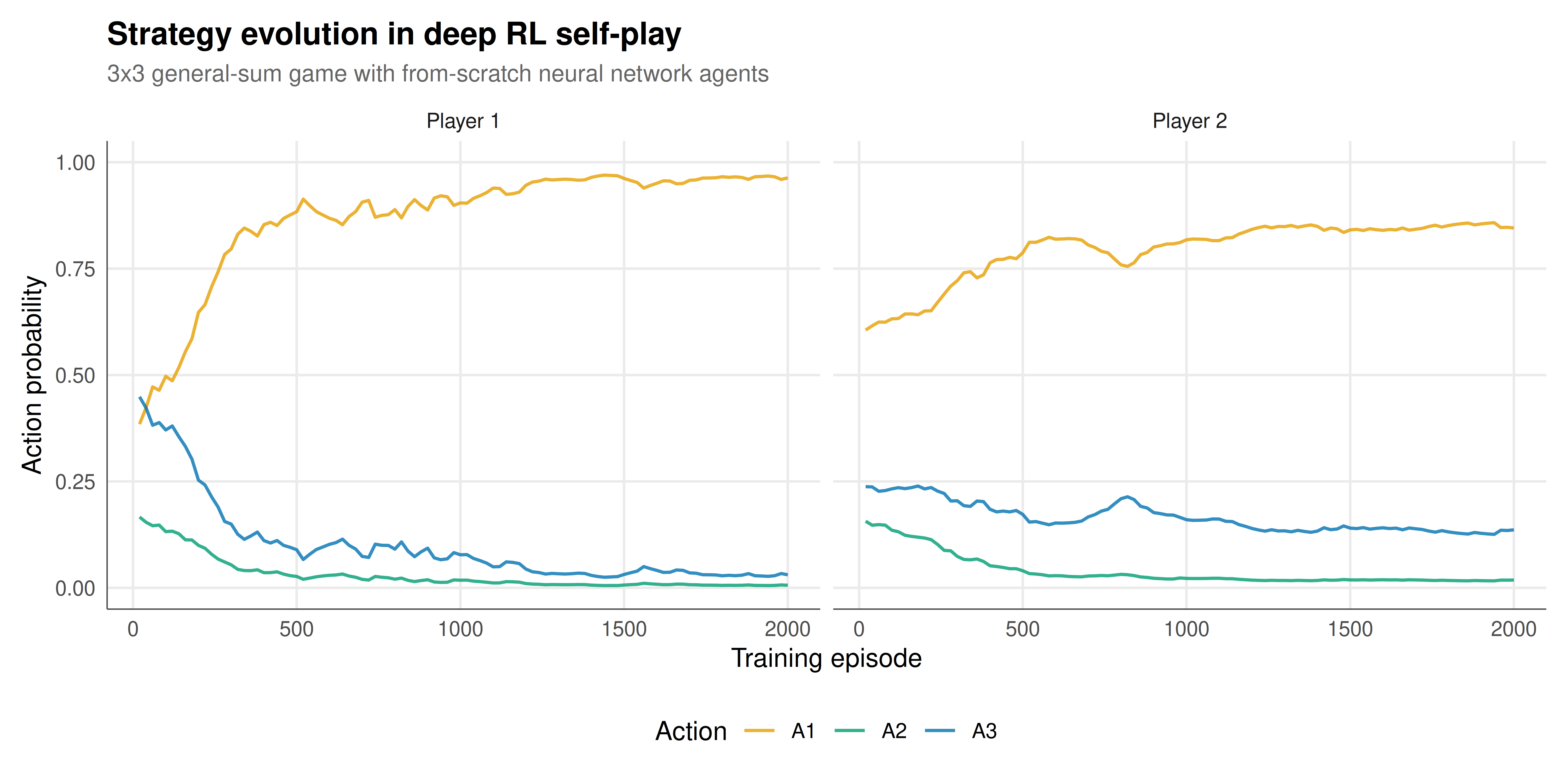
The figure tracks how each agent’s mixed strategy evolves over training episodes, showing convergence behavior relative to the game’s strategic structure.

p_static <- ggplot(strategy_history,
                   aes(x = episode, y = prob, color = action)) +
  geom_line(linewidth = 0.7, alpha = 0.8) +
  facet_wrap(~ player) +
  scale_color_manual(values = okabe_ito[c(1, 3, 5)],
                     name = "Action") +
  labs(title = "Strategy evolution in deep RL self-play",
       subtitle = "3x3 general-sum game with from-scratch neural network agents",
       x = "Training episode", y = "Action probability") +
  ylim(0, 1) +
  theme_publication()

p_static

Figure 1: Evolution of learned mixed strategies during deep RL self-play on a 3x3 general-sum game. Each panel shows one player’s probability distribution over three actions as training progresses. The neural networks (16 hidden units, ReLU activation) are trained with Q-learning using softmax exploration. Strategy profiles oscillate as agents adapt to each other’s changing policies – a characteristic feature of multi-agent learning. Okabe-Ito palette.

Interactive figure

The interactive version displays exact probability values and Q-value-derived policy details on hover for each recorded training step.

strat_int <- strategy_history %>%
  mutate(text_label = paste0("Episode: ", episode,
                             "\n", player,
                             "\nAction: ", action,
                             "\nProbability: ", round(prob, 4)))

p_int <- ggplot(strat_int,
                aes(x = episode, y = prob, color = action,
                    text = text_label)) +
  geom_line(linewidth = 0.6, alpha = 0.8) +
  facet_wrap(~ player) +
  scale_color_manual(values = okabe_ito[c(1, 3, 5)],
                     name = "Action") +
  labs(title = "Strategy evolution (interactive)",
       x = "Episode", y = "Probability") +
  ylim(0, 1) +
  theme_publication()

ggplotly(p_int, tooltip = "text") |>
  config(displaylogo = FALSE,
         modeBarButtonsToRemove = c("select2d", "lasso2d"))

Figure 2

Interpretation

The self-play training dynamics reveal several important phenomena at the intersection of deep reinforcement learning and game theory. Most strikingly, the agents’ strategy profiles do not converge smoothly to a fixed point as they would in single-agent RL. Instead, they exhibit oscillatory behavior: as Player 1 shifts toward action A1, Player 2 adapts by increasing the probability of its best response, which in turn causes Player 1 to adjust, creating a feedback loop of mutual adaptation. This cycling is not a bug in the implementation – it is a fundamental feature of independent learning in general-sum games, predicted by theoretical results on the non-convergence of gradient dynamics in non-zero-sum settings.

The game we selected (a modified Battle of the Sexes with a third “compromise” action) has a rich strategic structure. The pure-strategy Nash equilibria are at (A1, A1) and (A2, A2), where players coordinate on the same activity but with different preferences over which coordination point is selected. The third action A3 provides a safe option with moderate payoff regardless of the opponent’s choice. The mixed-strategy Nash equilibrium involves positive probability on all three actions, but the exact mixing probabilities depend on the payoff values. Our deep RL agents explore this landscape through trial and error, gradually learning that actions A1 and A2 yield high rewards when coordinated but zero otherwise, while A3 provides a consistent fallback.

The neural network architecture we implemented from scratch – a single hidden layer with 16 ReLU units – is deliberately minimal. This transparency serves a pedagogical purpose: every matrix multiplication, every gradient computation, and every weight update is visible in the code. The forward pass computes \(Q(s, a) = W_2 \cdot \text{ReLU}(W_1 s + b_1) + b_2\), producing three Q-values that are transformed into action probabilities via softmax. The backward pass computes gradients of the temporal difference error with respect to each parameter layer. Despite its simplicity, this network has sufficient capacity to represent arbitrary Q-value functions over three actions, which is all that is needed for a single-state matrix game.

The temperature parameter in the softmax policy plays a critical role in the learning dynamics. We anneal the temperature from 1.0 to 0.3 over training, initially encouraging exploration (near-uniform action probabilities) and gradually shifting to exploitation (concentrating probability on high-Q actions). If the temperature is too high throughout training, the agents never commit to any strategy and the Q-values remain noisy. If the temperature is too low from the start, the agents commit prematurely to a pure strategy (whichever action happens to receive positive reinforcement first) and may lock into a non-equilibrium outcome. The annealing schedule thus serves a function analogous to the cooling schedule in simulated annealing – balancing exploration and exploitation.

An important limitation of independent Q-learning for games is that each agent treats the other as part of the environment, ignoring the fact that the other agent is also learning. This can lead to convergence failures even in simple games. More sophisticated approaches such as policy gradient with opponent modeling, or centralized training with decentralized execution, address this limitation but require substantially more complex implementations. Our from-scratch approach provides the foundation for understanding these advanced methods by making the basic learning mechanism fully transparent.

Extensions & related tutorials

Deep RL for games connects to several related approaches for learning in strategic environments.

• Fictitious play convergence
• No-regret learning in games
• Multi-agent reinforcement learning
• Simulated annealing for equilibrium computation

References