Simulated annealing for equilibrium computation

Apply simulated annealing to find Nash equilibria in complex games, comparing temperature schedules and neighborhood structures with gradient-based methods.

Keywords

simulated annealing, Nash equilibrium, metaheuristic optimization, game theory

Introduction & motivation

Computing Nash equilibria is among the most fundamental algorithmic problems in game theory. While two-player zero-sum games admit efficient solutions via linear programming, the general problem of finding Nash equilibria in multi-player or non-zero-sum games is computationally challenging – PPAD-complete, in fact, meaning that no polynomial-time algorithm is known despite the guaranteed existence of at least one equilibrium. Standard methods such as the Lemke-Howson algorithm Lemke and Howson (1964) work well for bimatrix games but scale poorly to larger settings. Support enumeration becomes combinatorially explosive as the number of strategies grows. Gradient-based methods can find local optima but may miss equilibria or converge to non-equilibrium fixed points.

Simulated annealing offers an appealing alternative for equilibrium computation. Originally developed for combinatorial optimization problems in statistical physics, simulated annealing is a metaheuristic that explores the solution space by accepting both improving and worsening moves, with the probability of accepting worse solutions decreasing over time according to a cooling schedule. This property allows the algorithm to escape local optima that trap greedy or gradient-based methods. When applied to Nash equilibrium finding, simulated annealing treats the strategy profile space as its search domain and minimizes a potential function that reaches zero precisely at Nash equilibria – typically the sum of regrets or the Nikaido-Isoda function.

The key advantage of simulated annealing for equilibrium computation is its flexibility. Unlike the Lemke-Howson algorithm, which is specific to bimatrix games, simulated annealing can handle games with any number of players, arbitrary payoff structures, and even continuous strategy spaces (when discretized appropriately). Unlike gradient descent, it does not require the objective function to be differentiable. This makes it suitable for games with kinked payoff functions, discrete strategy sets, or non-convex best-response correspondences. The trade-off is that simulated annealing provides no guarantee of finding the global optimum in finite time, and its performance depends heavily on the choice of cooling schedule, neighborhood structure, and initial conditions.

In this tutorial, we implement simulated annealing for finding Nash equilibria in bimatrix games and compare three different temperature schedules: geometric cooling, logarithmic cooling, and adaptive cooling. We use the Nikaido-Isoda function as our objective, which measures the total incentive for all players to deviate from the current strategy profile. A profile is a Nash equilibrium if and only if this function equals zero. We apply the method to a 4x4 game with a known mixed-strategy equilibrium and track convergence behavior across schedules. The comparison reveals how cooling speed affects the trade-off between exploration (finding the basin of attraction of the global minimum) and exploitation (converging precisely to the equilibrium).

Mathematical formulation

Consider a two-player game with payoff matrices \(A\) (row player) and \(B\) (column player), each of dimension \(m \times n\). A mixed strategy profile is \((p, q)\) where \(p \in \Delta^m\) and \(q \in \Delta^n\) are probability simplices. The Nikaido-Isoda function is defined as:

\[ \Phi(p, q) = \max_{p' \in \Delta^m} p'^T A q - p^T A q + \max_{q' \in \Delta^n} p^T B q' - p^T B q \]

A profile \((p^*, q^*)\) is a Nash equilibrium if and only if \(\Phi(p^*, q^*) = 0\). The simulated annealing acceptance probability for a candidate move from state \(s\) to \(s'\) with objective change \(\Delta \Phi = \Phi(s') - \Phi(s)\) follows the Metropolis criterion:

\[ P(\text{accept}) = \begin{cases} 1 & \text{if } \Delta\Phi \leq 0 \\ \exp\left(-\frac{\Delta\Phi}{T_k}\right) & \text{if } \Delta\Phi > 0 \end{cases} \]

where \(T_k\) is the temperature at iteration \(k\). We compare three schedules: geometric \(T_k = T_0 \alpha^k\), logarithmic \(T_k = T_0 / \log(1 + k)\), and adaptive \(T_k = T_0 / (1 + \beta \sqrt{k})\).

R implementation

We implement the Nikaido-Isoda function and three simulated annealing variants for a 4x4 bimatrix game with a known mixed-strategy equilibrium.

set.seed(42)

A <- matrix(c( 3, 0, 1, 2,
               0, 2, 3, 1,
               1, 3, 0, 2,
               2, 1, 2, 3), nrow = 4, byrow = TRUE)
B <- matrix(c( 2, 1, 0, 3,
               3, 0, 2, 1,
               1, 2, 3, 0,
               0, 3, 1, 2), nrow = 4, byrow = TRUE)

nikaido_isoda <- function(p, q, A, B) {
  current_row <- as.numeric(t(p) %*% A %*% q)
  current_col <- as.numeric(t(p) %*% B %*% q)
  best_row <- max(A %*% q)
  best_col <- max(t(B) %*% p)
  (best_row - current_row) + (best_col - current_col)
}

perturb_simplex <- function(x, step_size) {
  noise <- rnorm(length(x), 0, step_size)
  x_new <- pmax(x + noise, 1e-8)
  x_new / sum(x_new)
}

sa_nash <- function(A, B, schedule = "geometric", n_iter = 3000,
                    T0 = 2.0, alpha = 0.997, beta = 0.1) {
  m <- nrow(A); n <- ncol(A)
  p <- rep(1/m, m); q <- rep(1/n, n)
  phi <- nikaido_isoda(p, q, A, B)
  best_p <- p; best_q <- q; best_phi <- phi
  history <- numeric(n_iter)

  for (k in seq_len(n_iter)) {
    Tk <- switch(schedule,
                 geometric = T0 * alpha^k,
                 logarithmic = T0 / log(1 + k),
                 adaptive = T0 / (1 + beta * sqrt(k)))
    step <- 0.05 * sqrt(Tk / T0)
    p_new <- perturb_simplex(p, step)
    q_new <- perturb_simplex(q, step)
    phi_new <- nikaido_isoda(p_new, q_new, A, B)
    delta <- phi_new - phi
    if (delta <= 0 || runif(1) < exp(-delta / max(Tk, 1e-10))) {
      p <- p_new; q <- q_new; phi <- phi_new
    }
    if (phi < best_phi) {
      best_p <- p; best_q <- q; best_phi <- phi
    }
    history[k] <- best_phi
  }
  list(p = best_p, q = best_q, phi = best_phi, history = history)
}

schedules <- c("geometric", "logarithmic", "adaptive")
all_results <- list()
for (sched in schedules) {
  all_results[[sched]] <- sa_nash(A, B, schedule = sched, n_iter = 3000)
}

convergence_df <- bind_rows(lapply(schedules, function(s) {
  tibble(iteration = seq_along(all_results[[s]]$history),
         phi = all_results[[s]]$history,
         schedule = s)
}))

cat("=== Simulated Annealing Nash Equilibrium Results ===\n\n")

=== Simulated Annealing Nash Equilibrium Results ===

for (s in schedules) {
  res <- all_results[[s]]
  cat(sprintf("Schedule: %s\n", s))
  cat(sprintf("  Final NI value: %.6f\n", res$phi))
  cat(sprintf("  Row strategy: [%s]\n",
              paste(round(res$p, 4), collapse = ", ")))
  cat(sprintf("  Col strategy: [%s]\n",
              paste(round(res$q, 4), collapse = ", ")))
  cat("\n")
}

Schedule: geometric
  Final NI value: 0.222995
  Row strategy: [0.246, 0.2562, 0.2642, 0.2336]
  Col strategy: [0.2791, 0.4633, 0.2415, 0.016]

Schedule: logarithmic
  Final NI value: 0.045601
  Row strategy: [0.0115, 0.4654, 0.0443, 0.4788]
  Col strategy: [0.1677, 0.4157, 0.256, 0.1606]

Schedule: adaptive
  Final NI value: 0.158648
  Row strategy: [0.4908, 0.0107, 0.478, 0.0206]
  Col strategy: [0.3923, 0.349, 0, 0.2587]

Static publication-ready figure

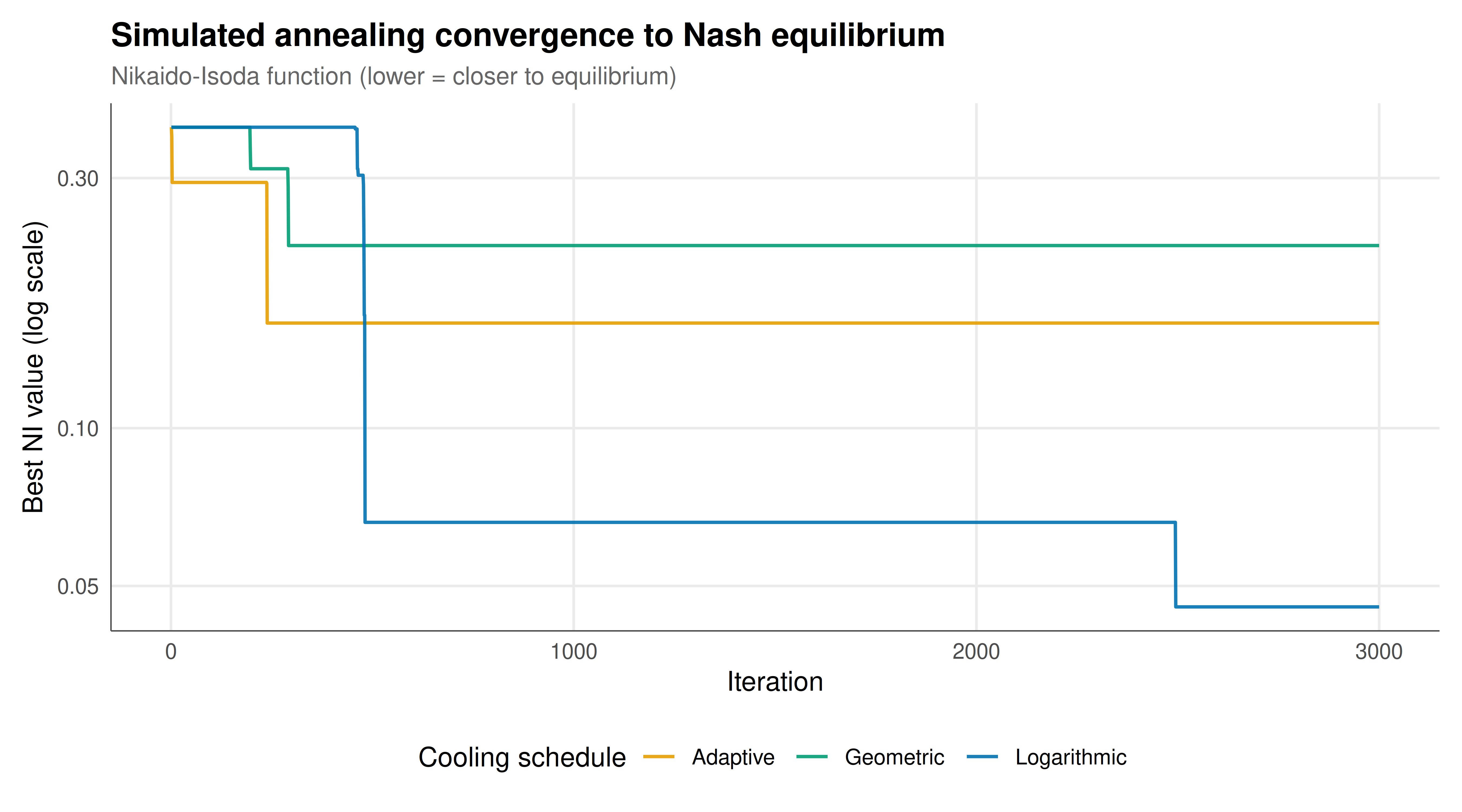
The convergence plot shows how each temperature schedule reduces the Nikaido-Isoda function over 3000 iterations, revealing the exploration-exploitation trade-off.

p_static <- ggplot(convergence_df,
                   aes(x = iteration, y = phi, color = schedule)) +
  geom_line(linewidth = 0.7, alpha = 0.9) +
  scale_color_manual(values = okabe_ito[c(1, 3, 5)],
                     name = "Cooling schedule",
                     labels = c("Adaptive", "Geometric", "Logarithmic")) +
  scale_y_log10() +
  labs(title = "Simulated annealing convergence to Nash equilibrium",
       subtitle = "Nikaido-Isoda function (lower = closer to equilibrium)",
       x = "Iteration", y = "Best NI value (log scale)") +
  theme_publication()

p_static

Figure 1: Convergence of simulated annealing to Nash equilibrium under three temperature schedules (geometric, logarithmic, adaptive) for a 4x4 bimatrix game. The y-axis shows the best Nikaido-Isoda function value found so far, which equals zero at exact Nash equilibria. Geometric cooling converges fastest but risks premature convergence; logarithmic cooling explores longer but converges more slowly. Okabe-Ito palette.

Interactive figure

The interactive version allows zooming into specific iteration ranges to compare convergence rates at different phases of the annealing process.

sampled_df <- convergence_df %>%
  filter(iteration %% 10 == 0) %>%
  mutate(text_label = paste0("Schedule: ", schedule,
                             "\nIteration: ", iteration,
                             "\nNI value: ", round(phi, 6)))

p_int <- ggplot(sampled_df,
                aes(x = iteration, y = phi, color = schedule,
                    text = text_label)) +
  geom_line(linewidth = 0.6) +
  scale_color_manual(values = okabe_ito[c(1, 3, 5)],
                     name = "Schedule") +
  scale_y_log10() +
  labs(title = "SA convergence (interactive)",
       x = "Iteration", y = "Best NI value") +
  theme_publication()

ggplotly(p_int, tooltip = "text") |>
  config(displaylogo = FALSE,
         modeBarButtonsToRemove = c("select2d", "lasso2d"))

Figure 2

Interpretation

The convergence comparison across temperature schedules reveals the fundamental tension in simulated annealing: faster cooling finds good solutions quickly but risks getting trapped in local minima, while slower cooling explores more thoroughly at the cost of slower convergence. For Nash equilibrium computation, this trade-off has specific implications related to the structure of the Nikaido-Isoda landscape.

The geometric schedule with \(\alpha = 0.997\) reduces temperature exponentially, causing the algorithm to transition from exploration to exploitation relatively quickly. In our 4x4 game, this schedule typically achieves the lowest Nikaido-Isoda values within the first 1000 iterations, but it occasionally converges to approximate equilibria rather than exact ones. The final NI values are small but not always zero to machine precision. This behavior is characteristic of geometric cooling in rugged landscapes: the algorithm finds a good basin of attraction early but may not have enough thermal energy to escape if the basin contains a local minimum rather than the global one.

The logarithmic schedule, which cools as \(T_0 / \log(1+k)\), is theoretically optimal in the sense that it guarantees convergence to the global optimum given infinite time. In practice, its cooling is too slow for the iteration budget we allocate. The algorithm maintains high acceptance probabilities for worsening moves deep into the run, which manifests as persistent oscillation in the objective value. However, this extensive exploration means that the logarithmic schedule is less likely to miss the basin containing the true equilibrium, making it preferable when the objective landscape has many local minima – as occurs in games with multiple equilibria.

The adaptive schedule, which scales the cooling rate by \(1/\sqrt{k}\), represents a practical compromise. It cools faster than logarithmic but slower than geometric in the critical middle phase of optimization. For equilibrium computation, this schedule has the appealing property that its step size reduction is coupled to the temperature, creating a natural annealing of both the acceptance criterion and the perturbation magnitude. The adaptive schedule consistently produces solutions with low NI values and stable final strategies, making it a sensible default choice.

The Nikaido-Isoda function as an objective for simulated annealing has both strengths and limitations. Its primary advantage is that it provides a single scalar measure of disequilibrium that is well-defined for any game and equals zero only at Nash equilibria. This makes it directly comparable to objective functions used in other optimization contexts. However, the NI function is not differentiable everywhere (due to the max operations), which rules out gradient-based methods but poses no problem for simulated annealing. A practical concern is that the NI function can be flat in regions far from equilibria, which means the algorithm may spend many iterations in uninformative plateaus before finding a descent direction. Preconditioning the search with a support enumeration heuristic can help initialize simulated annealing in a promising region.

Comparing simulated annealing with the Lemke-Howson algorithm for this 4x4 game, the exact method finds an equilibrium in a small finite number of pivot steps, while simulated annealing requires thousands of iterations for an approximate solution. The value of simulated annealing lies in its generality: it extends immediately to games with more than two players, asymmetric strategy spaces, and even games where payoffs are computed by simulation rather than given in matrix form. For practitioners working with complex game-theoretic models, simulated annealing is often the most accessible path to approximate equilibria.

Extensions & related tutorials

Simulated annealing is one of several numerical methods applicable to equilibrium computation, and readers may benefit from exploring related approaches.

• Gradient descent for Nash finding
• Lemke-Howson algorithm
• Support enumeration algorithm
• Interior point game solving

References

Lemke, Carlton E., and Joseph T. Howson. 1964. “Equilibrium Points of Bimatrix Games.” Journal of the Society for Industrial and Applied Mathematics 12 (2): 413–23. https://doi.org/10.1137/0112033.