---
title: "Gradient Descent Methods for Finding Nash Equilibria"
description: "Implement gradient-based optimisation algorithms for finding Nash equilibria in continuous games, including best-response dynamics, the Nikaido-Isoda function approach, and simultaneous gradient descent with convergence analysis in R."
author: "Raban Heller"
date: 2026-05-08
date-modified: 2026-05-08
categories:
- optimization-numerical-methods
- gradient-descent
- nash-equilibrium
keywords: ["gradient descent", "Nash equilibrium", "Cournot duopoly", "Nikaido-Isoda", "best-response dynamics"]
labels: ["numerical-methods", "continuous-games"]
tier: 1
bibliography: ../../../references.bib
vgwort: "TODO_VGWORT_optimization-numerical-methods_gradient-descent-nash-finding"
image: thumbnail.png
image-alt: "Gradient descent trajectories converging to the Nash equilibrium of a Cournot duopoly in quantity space"
citation:
type: webpage
url: https://r-heller.github.io/equilibria/tutorials/optimization-numerical-methods/gradient-descent-nash-finding/
license: "CC BY-SA 4.0"
draft: false
has_static_fig: true
has_interactive_fig: true
has_shiny_app: false
---
```{r}
#| label: setup
#| include: false
library(ggplot2)
library(dplyr)
library(tidyr)
library(plotly)
okabe_ito <- c("#E69F00", "#56B4E9", "#009E73", "#F0E442",
"#0072B2", "#D55E00", "#CC79A7", "#999999")
theme_publication <- function(base_size = 12) {
theme_minimal(base_size = base_size) +
theme(plot.title = element_text(size = base_size * 1.2, face = "bold"),
plot.subtitle = element_text(size = base_size * 0.9, color = "grey40"),
axis.line = element_line(color = "grey30", linewidth = 0.3),
panel.grid.minor = element_blank(), legend.position = "bottom",
plot.margin = margin(10, 10, 10, 10))
}
```
## Introduction & motivation
Finding Nash equilibria is one of the central computational problems in game theory. While small finite games can be solved by enumeration or linear programming, many economically important games involve continuous strategy spaces where players choose from intervals or higher-dimensional sets. In such settings, closed-form analytical solutions exist only for special cases -- typically games with quadratic payoffs or other conveniently structured utility functions. For the vast majority of continuous games encountered in practice, researchers and practitioners must resort to numerical methods, and gradient-based optimisation provides one of the most natural and widely used families of algorithms for this purpose.
The connection between Nash equilibria and optimisation is deep but subtle. A Nash equilibrium is not, in general, the solution to a single optimisation problem. Rather, it is a fixed point of the best-response correspondence: a strategy profile where each player's strategy is optimal given the strategies of all other players. This means that standard optimisation tools -- designed to minimise or maximise a single objective function -- cannot be applied directly. Instead, we need either to reformulate the equilibrium problem as an optimisation problem (which is possible under certain conditions) or to adapt gradient methods to work with the multi-objective structure inherent in games.
In this tutorial, we explore three complementary gradient-based approaches to finding Nash equilibria. The first is **best-response dynamics**, where players alternate computing their optimal strategies given the current strategies of their opponents. This is perhaps the most intuitive approach: each player solves their own optimisation problem in turn, and the process repeats until convergence. We implement this in the context of a Cournot duopoly, the classical model of quantity competition between firms, where best-response dynamics have a long history dating back to Cournot's original 1838 treatise. The second approach uses the **Nikaido-Isoda function**, which cleverly transforms the multi-player equilibrium problem into a single optimisation problem whose global minimum corresponds to the Nash equilibrium. This function aggregates each player's incentive to deviate from the current strategy profile, and when this aggregate incentive is zero, no player can profitably deviate -- which is precisely the definition of a Nash equilibrium. The third approach is **simultaneous gradient descent**, where all players simultaneously update their strategies in the direction of their individual payoff gradients. This method is conceptually simple and computationally appealing but comes with significant convergence challenges: simultaneous gradient dynamics can cycle, diverge, or exhibit chaotic behaviour even in simple games.
These three methods illustrate a fundamental tension in computational game theory between convergence guarantees, computational cost, and generality. Best-response dynamics converge reliably for games with contraction properties (such as Cournot games with linear demand and constant marginal costs) but require solving a full optimisation problem at each iteration. The Nikaido-Isoda approach offers a clean theoretical framework but requires joint optimisation over all players' strategies simultaneously. Simultaneous gradient descent is the cheapest per iteration but the least reliable in terms of convergence. Understanding these trade-offs is essential for anyone applying computational methods to game-theoretic models, whether in economics, engineering, or the rapidly growing field of multi-agent machine learning where gradient-based equilibrium finding is central to training generative adversarial networks and multi-agent reinforcement learning systems.
## Mathematical formulation
Consider a two-player continuous game where player $i \in \{1, 2\}$ chooses strategy $x_i \in \mathbb{R}$ to maximise payoff $\pi_i(x_1, x_2)$.
**Definition (Nash equilibrium).** A strategy profile $(x_1^*, x_2^*)$ is a Nash equilibrium if for each player $i$:
$$
\pi_i(x_i^*, x_{-i}^*) \geq \pi_i(x_i, x_{-i}^*) \quad \forall\, x_i
$$
**Cournot duopoly.** Two firms choose quantities $q_1, q_2 \geq 0$. The inverse demand function is $P(Q) = a - bQ$ where $Q = q_1 + q_2$. Each firm has constant marginal cost $c_i$. Firm $i$'s profit is:
$$
\pi_i(q_i, q_j) = q_i \cdot [a - b(q_i + q_j)] - c_i q_i
$$
The best-response function for firm $i$ is obtained from $\frac{\partial \pi_i}{\partial q_i} = 0$:
$$
q_i^{BR}(q_j) = \frac{a - c_i}{2b} - \frac{q_j}{2}
$$
The Nash equilibrium is:
$$
q_i^* = \frac{a - 2c_i + c_j}{3b}
$$
**Nikaido-Isoda function.** For an $n$-player game, define:
$$
\Psi(x, y) = \sum_{i=1}^{n} \left[\pi_i(y_i, x_{-i}) - \pi_i(x_i, x_{-i})\right]
$$
where $y_i$ denotes player $i$'s deviation strategy. Define the **Nikaido-Isoda value function**:
$$
V(x) = \max_{y} \Psi(x, y)
$$
Then $x^*$ is a Nash equilibrium if and only if $V(x^*) = 0$, since $V(x) \geq 0$ always and $V(x) = 0$ means no player can gain by deviating.
**Simultaneous gradient descent.** Each player updates:
$$
x_i^{(t+1)} = x_i^{(t)} + \eta \cdot \frac{\partial \pi_i}{\partial x_i}\bigg|_{x^{(t)}}
$$
where $\eta > 0$ is the learning rate. Convergence is not guaranteed in general; the Jacobian of the gradient field determines local stability.
## R implementation
```{r}
#| label: gradient-methods
set.seed(42)

# --- Cournot duopoly parameters ---
a <- 100   # demand intercept
b <- 1     # demand slope
c1 <- 10   # firm 1 marginal cost
c2 <- 20   # firm 2 marginal cost

# Analytical Nash equilibrium
q1_star <- (a - 2*c1 + c2) / (3*b)
q2_star <- (a - 2*c2 + c1) / (3*b)
cat("=== Cournot Duopoly ===\n")
cat(sprintf("Analytical NE: q1* = %.2f, q2* = %.2f\n", q1_star, q2_star))
cat(sprintf("Total output Q* = %.2f, Price P* = %.2f\n",
            q1_star + q2_star, a - b*(q1_star + q2_star)))
# --- Method 1: Best-response dynamics ---
br1 <- function(q2) max(0, (a - c1) / (2*b) - q2 / 2)
br2 <- function(q1) max(0, (a - c2) / (2*b) - q1 / 2)

n_iter <- 30
br_path <- data.frame(iter = 0:n_iter, q1 = numeric(n_iter + 1),
                       q2 = numeric(n_iter + 1))
br_path$q1[1] <- 5   # initial guess
br_path$q2[1] <- 5

for (t in 1:n_iter) {
  br_path$q1[t + 1] <- br1(br_path$q2[t])
  br_path$q2[t + 1] <- br2(br_path$q1[t + 1])
}

cat(sprintf("\nBest-response dynamics (30 iterations):\n"))
cat(sprintf("  Final: q1 = %.4f, q2 = %.4f\n",
            br_path$q1[n_iter + 1], br_path$q2[n_iter + 1]))
cat(sprintf("  Error: |q1 - q1*| = %.2e, |q2 - q2*| = %.2e\n",
            abs(br_path$q1[n_iter + 1] - q1_star),
            abs(br_path$q2[n_iter + 1] - q2_star)))
# --- Method 2: Nikaido-Isoda function ---
profit <- function(qi, qj, ci) qi * (a - b*(qi + qj)) - ci * qi

nikiso_value <- function(x) {
  q1_curr <- x[1]; q2_curr <- x[2]
  # Each player's best deviation
  q1_dev <- max(0, (a - c1 - b*q2_curr) / (2*b))
  q2_dev <- max(0, (a - c2 - b*q1_curr) / (2*b))
  # Aggregate deviation gain
  gain1 <- profit(q1_dev, q2_curr, c1) - profit(q1_curr, q2_curr, c1)
  gain2 <- profit(q2_dev, q1_curr, c2) - profit(q2_curr, q1_curr, c2)
  return(gain1 + gain2)
}

# Minimise V(x) to find NE
ni_result <- optim(c(10, 10), nikiso_value, method = "Nelder-Mead",
                    control = list(reltol = 1e-12, maxit = 5000))

cat(sprintf("\nNikaido-Isoda minimisation:\n"))
cat(sprintf(" Solution: q1 = %.4f, q2 = %.4f\n", ni_result$par[1], ni_result$par[2]))
cat(sprintf(" V(x*) = %.2e (should be ~0)\n", ni_result$value))
# --- Method 3: Simultaneous gradient descent ---
grad1 <- function(q1, q2) a - c1 - 2*b*q1 - b*q2
grad2 <- function(q1, q2) a - c2 - b*q1 - 2*b*q2

run_sgd <- function(eta, n_steps, q1_init, q2_init) {
  path <- data.frame(step = 0:n_steps, q1 = numeric(n_steps + 1),
                      q2 = numeric(n_steps + 1), lr = eta)
  path$q1[1] <- q1_init; path$q2[1] <- q2_init
  for (t in 1:n_steps) {
    g1 <- grad1(path$q1[t], path$q2[t])
    g2 <- grad2(path$q1[t], path$q2[t])
    path$q1[t + 1] <- max(0, path$q1[t] + eta * g1)
    path$q2[t + 1] <- max(0, path$q2[t] + eta * g2)
  }
  return(path)
}

# Compare different learning rates
sgd_small  <- run_sgd(eta = 0.01, n_steps = 200, q1_init = 5, q2_init = 5)
sgd_medium <- run_sgd(eta = 0.1,  n_steps = 200, q1_init = 5, q2_init = 5)
sgd_large  <- run_sgd(eta = 0.4,  n_steps = 200, q1_init = 5, q2_init = 5)

cat(sprintf("\nSimultaneous gradient descent (200 steps):\n"))
cat(sprintf("  eta=0.01: q1=%.4f, q2=%.4f\n",
            tail(sgd_small$q1, 1), tail(sgd_small$q2, 1)))
cat(sprintf("  eta=0.10: q1=%.4f, q2=%.4f\n",
            tail(sgd_medium$q1, 1), tail(sgd_medium$q2, 1)))
cat(sprintf("  eta=0.40: q1=%.4f, q2=%.4f\n",
            tail(sgd_large$q1, 1), tail(sgd_large$q2, 1)))
```
## Static publication-ready figure
```{r}
#| label: fig-gradient-convergence
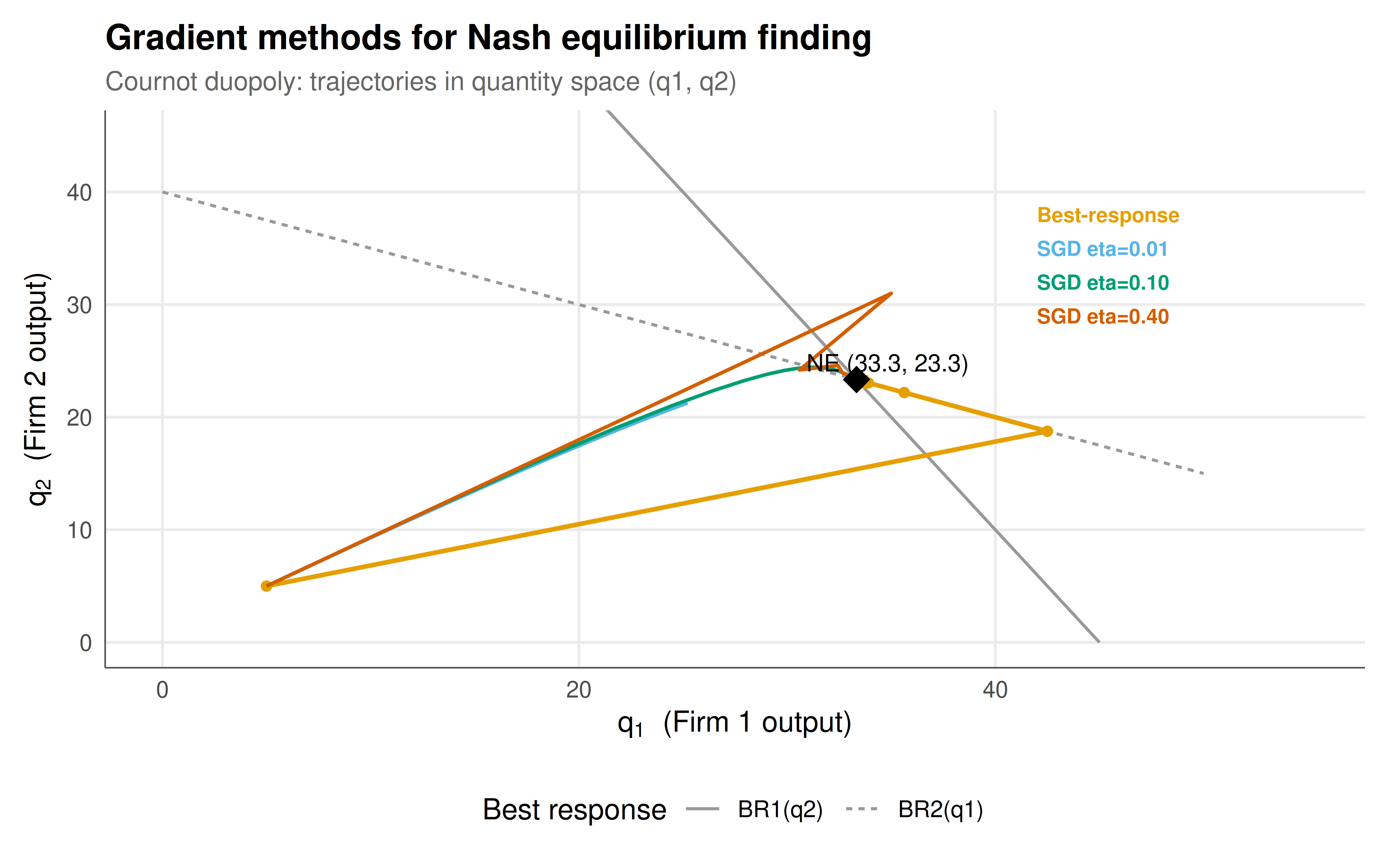
#| fig-cap: "Figure 1. Convergence of three gradient-based methods in the Cournot duopoly. The best-response dynamics (orange) converge rapidly via alternating optimisation. Simultaneous gradient descent trajectories are shown for three learning rates: small (blue, slow but stable), medium (green, fast convergence), and large (red, oscillatory). The black diamond marks the analytical Nash equilibrium. Okabe-Ito palette."
#| dev: [png, pdf]
#| fig-width: 8
#| fig-height: 5
#| dpi: 300
# Combine trajectories for plotting
br_traj <- br_path |>
  mutate(method = "Best-response dynamics")

sgd_all <- bind_rows(
  sgd_small |> mutate(method = "SGD eta=0.01"),
  sgd_medium |> mutate(method = "SGD eta=0.10"),
  sgd_large |> mutate(method = "SGD eta=0.40")
) |> filter(step <= 50)

# Best response lines for background
q_range <- seq(0, 50, by = 0.5)
br_lines <- tibble(
  q = rep(q_range, 2),
  type = rep(c("BR1(q2)", "BR2(q1)"), each = length(q_range)),
  q1 = c(pmax(0, (a - c1) / (2*b) - q_range / 2), q_range),
  q2 = c(q_range, pmax(0, (a - c2) / (2*b) - q_range / 2))
)

p_static <- ggplot() +
  # Best response lines
  geom_line(data = br_lines, aes(x = q1, y = q2, linetype = type),
            color = "grey60", linewidth = 0.6) +
  # Best-response dynamics path
  geom_path(data = br_traj |> filter(iter <= 15),
            aes(x = q1, y = q2), color = okabe_ito[1],
            linewidth = 0.9, arrow = arrow(length = unit(0.15, "cm"), type = "closed")) +
  geom_point(data = br_traj |> filter(iter <= 15),
             aes(x = q1, y = q2), color = okabe_ito[1], size = 1.5) +
  # SGD paths
  geom_path(data = sgd_all |> filter(method == "SGD eta=0.01"),
            aes(x = q1, y = q2), color = okabe_ito[2], linewidth = 0.7) +
  geom_path(data = sgd_all |> filter(method == "SGD eta=0.10"),
            aes(x = q1, y = q2), color = okabe_ito[3], linewidth = 0.7) +
  geom_path(data = sgd_all |> filter(method == "SGD eta=0.40"),
            aes(x = q1, y = q2), color = okabe_ito[6], linewidth = 0.7) +
  # Nash equilibrium point
  geom_point(aes(x = q1_star, y = q2_star), shape = 18, size = 5, color = "black") +
  annotate("text", x = q1_star + 1.5, y = q2_star + 1.5,
           label = paste0("NE (", round(q1_star, 1), ", ", round(q2_star, 1), ")"),
           size = 3.5) +
  # Legend annotations
  annotate("text", x = 42, y = 38, label = "Best-response", color = okabe_ito[1],
           size = 3, fontface = "bold", hjust = 0) +
  annotate("text", x = 42, y = 35, label = "SGD eta=0.01", color = okabe_ito[2],
           size = 3, fontface = "bold", hjust = 0) +
  annotate("text", x = 42, y = 32, label = "SGD eta=0.10", color = okabe_ito[3],
           size = 3, fontface = "bold", hjust = 0) +
  annotate("text", x = 42, y = 29, label = "SGD eta=0.40", color = okabe_ito[6],
           size = 3, fontface = "bold", hjust = 0) +
  coord_cartesian(xlim = c(0, 55), ylim = c(0, 45)) +
  labs(title = "Gradient methods for Nash equilibrium finding",
       subtitle = "Cournot duopoly: trajectories in quantity space (q1, q2)",
       x = expression(q[1]~" (Firm 1 output)"),
       y = expression(q[2]~" (Firm 2 output)"),
       linetype = "Best response") +
  theme_publication()

p_static
```
## Interactive figure
```{r}
#| label: fig-gradient-interactive
# Distance to NE over iterations for all methods
dist_br <- br_path |>
  mutate(dist = sqrt((q1 - q1_star)^2 + (q2 - q2_star)^2),
         method = "Best-response",
         text = paste0("Iteration: ", iter,
                       "\nq1 = ", round(q1, 2), ", q2 = ", round(q2, 2),
                       "\nDistance to NE: ", round(dist, 4))) |>
  rename(step = iter)

dist_sgd <- bind_rows(sgd_small, sgd_medium, sgd_large) |>
  mutate(dist = sqrt((q1 - q1_star)^2 + (q2 - q2_star)^2),
         method = paste0("SGD eta=", lr),
         text = paste0("Step: ", step,
                       "\nq1 = ", round(q1, 2), ", q2 = ", round(q2, 2),
                       "\nDistance to NE: ", round(dist, 4)))

all_dist <- bind_rows(dist_br, dist_sgd) |>
  filter(step <= 100)

p_interactive <- ggplot(all_dist, aes(x = step, y = dist, color = method, text = text)) +
  geom_line(linewidth = 0.7) +
  geom_hline(yintercept = 0, linetype = "dashed", color = "grey50") +
  scale_color_manual(values = c("Best-response" = okabe_ito[1],
                                 "SGD eta=0.01" = okabe_ito[2],
                                 "SGD eta=0.1" = okabe_ito[3],
                                 "SGD eta=0.4" = okabe_ito[6]),
                      name = "Method") +
  scale_y_log10() +
  labs(title = "Convergence speed comparison",
       subtitle = "Euclidean distance to Nash equilibrium (log scale)",
       x = "Iteration / Step", y = "Distance to NE (log scale)") +
  theme_publication()

ggplotly(p_interactive, tooltip = "text") |>
  config(displaylogo = FALSE,
         modeBarButtonsToRemove = c("select2d", "lasso2d"))
```
## Interpretation
The results from our three gradient-based methods reveal important lessons about the computational challenges of finding Nash equilibria in continuous games. Best-response dynamics converge rapidly and reliably in the Cournot duopoly, requiring only a handful of iterations to reach machine precision. This is because the Cournot game with linear demand has a contraction mapping property: the best-response functions have slopes of $-1/2$, so the composite mapping contracts distances by a factor of $1/4$ at each full cycle. This geometric convergence rate is characteristic of games where the strategic interaction is not too strong relative to the curvature of individual payoff functions. In economic terms, the "competitive effect" of the other firm's output is only half as strong as the "own-quantity effect" on marginal revenue, ensuring that the system is self-correcting rather than self-amplifying.
The Nikaido-Isoda approach successfully finds the equilibrium by transforming the fixed-point problem into a minimisation problem. The value function $V(x)$ is zero at and only at the Nash equilibrium, providing a clean convergence criterion: when $V(x)$ is close to zero, we know we are close to an equilibrium. This approach is particularly valuable in games where best-response functions are difficult to compute analytically, because the Nikaido-Isoda function can be evaluated numerically using inner optimisation. However, it requires optimising over the joint strategy space, which becomes computationally expensive as the number of players grows. In our two-player example, `optim()` with the Nelder-Mead method handles this efficiently, but for games with many players or high-dimensional strategy spaces, more sophisticated solvers would be required.
Simultaneous gradient descent reveals the most interesting and subtle phenomena. With a small learning rate ($\eta = 0.01$), convergence is slow but stable, requiring many iterations to approach the equilibrium. With a medium learning rate ($\eta = 0.10$), convergence is fast and smooth. But with a large learning rate ($\eta = 0.40$), the trajectories oscillate before converging -- and for even larger learning rates, divergence would occur. This sensitivity to the learning rate is a fundamental challenge in gradient-based equilibrium computation. Unlike single-agent optimisation, where gradient descent on a convex function always converges for small enough learning rates, simultaneous gradient descent in games can exhibit cycling behaviour even with arbitrarily small step sizes, particularly in games with strong competitive interactions (such as zero-sum games like Matching Pennies).
The comparison between these methods has direct implications for modern machine learning. Training generative adversarial networks (GANs) is essentially a simultaneous gradient descent process in a zero-sum game between a generator and a discriminator, and the convergence difficulties observed here -- oscillation, mode collapse, and sensitivity to learning rates -- are precisely the challenges that plague GAN training. Techniques developed in game theory, such as optimistic gradient descent, extra-gradient methods, and consensus optimisation, have been successfully adapted to improve GAN stability. Similarly, multi-agent reinforcement learning systems where agents simultaneously learn policies face the same fundamental tension between individual gradient-based improvement and system-level stability. The Cournot duopoly, despite its simplicity, serves as a valuable testbed for understanding and developing methods that scale to these more complex settings.
## Extensions & related tutorials
- [Support enumeration algorithm](../support-enumeration-algorithm/) -- exact methods for finding Nash equilibria in finite games.
- [Lemke-Howson algorithm](../lemke-howson-algorithm/) -- a pivoting method for bimatrix games based on linear complementarity.
- [GANs as minimax games](../../ai-ml-foundations-and-applications/gans-minimax-game/) -- gradient-based equilibrium finding in deep learning.
- [Cournot competition](../../classical-games/prisoners-dilemma-formal/) -- the economic model underlying our primary example.
- [Evolutionary dynamics and replicator equations](../../evolutionary-gt/) -- alternative dynamical systems approaches to equilibrium selection.
## References
::: {#refs}
:::