Kaggle competitions as strategic interactions

Analyze Kaggle competitions through a game-theoretic lens, modeling competitor strategies, Nash equilibria of submission timing, and strategic model selection under competition rules.

Keywords

Kaggle, data science competition, Nash equilibrium, strategic model selection

Introduction & motivation

Kaggle competitions are commonly understood as machine learning benchmarks where participants optimize predictive accuracy on a held-out test set. But beneath the surface of gradient-boosted trees and neural network architectures lies a rich strategic environment. Each competitor must decide not only which models to build but when to submit, how many daily submissions to use, whether to form teams, and how much to rely on the public leaderboard for model selection. These decisions interact: a competitor who probes the leaderboard aggressively gains information but risks overfitting to the public test set, while a competitor who submits conservatively preserves generalization but may miss optimization opportunities. The resulting dynamics constitute a genuine multi-player game amenable to formal analysis.

The strategic structure of Kaggle competitions becomes clearest at the final submission stage. Most competitions allow participants to select a small number of final submissions (typically two) from their history. The private leaderboard, revealed only after the deadline, determines rankings and prizes. This creates a selection game: should a competitor choose the submission that scores highest on the public leaderboard, or hedge by selecting a more conservative model that might generalize better? The answer depends on what other competitors are likely to do. If most competitors chase the public leaderboard, then overfitting is widespread and a generalizing strategy gains relative advantage. If most competitors hedge, the public leaderboard becomes more informative and top-scoring submissions are more likely to hold up privately.

This tutorial models Kaggle competition dynamics as a series of strategic games. We begin with a two-player model of submission timing – should a competitor submit early (gaining information) or late (avoiding information leakage to rivals who monitor public scores)? We then extend to a model selection game where competitors choose between an aggressive high-variance model and a conservative low-variance model. Using simulated payoff matrices, we compute Nash equilibria and visualize the strategic landscape. The analysis reveals that the equilibrium strategies depend critically on the correlation between public and private test sets, the number of competitors, and the prize structure.

Real Kaggle competitions exhibit all the phenomena that game theory predicts. Leaderboard shakeups, where top public performers drop dramatically on the private board, are precisely the outcome of widespread overfitting – a coordination failure analogous to the Prisoner’s Dilemma. The formation of super-teams, where top competitors merge to pool diverse models, mirrors coalition formation in cooperative game theory. The Kaggle rule limiting daily submissions acts as a mechanism design constraint intended to reduce leaderboard probing, much like bid caps in auction design. By formalizing these dynamics, we can both explain observed competition outcomes and suggest strategies that account for opponent behavior.

Mathematical formulation

Consider a symmetric two-player game where each competitor chooses a strategy from \(\{A, C\}\): \(A\) (aggressive model, high variance) or \(C\) (conservative model, low variance). Let \(\rho\) denote the correlation between public and private test scores. The payoff matrix is:

\[ U = \begin{pmatrix} \rho \cdot v - (1-\rho) \cdot c & v \\ 0 & \rho \cdot v / 2 \end{pmatrix} \]

where \(v\) is the prize value and \(c\) is the overfitting penalty. Player 1 chooses rows; player 2 chooses columns. In the mixed-strategy Nash equilibrium, player \(i\) plays \(A\) with probability:

\[ p^* = \frac{\rho v / 2}{\rho v / 2 + (1-\rho) c} \]

For the submission timing game with \(n\) competitors and \(T\) rounds, the expected information gain from submitting in round \(t\) is:

\[ I(t) = \frac{T - t}{T} \cdot \sigma^2_{\text{public}} - \lambda \cdot \sum_{j \neq i} \mathbb{1}[\text{competitor } j \text{ observes score at } t] \]

where \(\lambda\) captures the information leakage cost.

R implementation

We simulate the model selection game across a range of public-private correlation values and compute Nash equilibrium mixing probabilities.

set.seed(42)

v <- 10
c_penalty <- 5
rho_values <- seq(0.1, 0.95, by = 0.05)

compute_nash <- function(rho, v, c_pen) {
  u_AA <- rho * v - (1 - rho) * c_pen
  u_AC <- v
  u_CA <- 0
  u_CC <- rho * v / 2
  p_star <- (u_CC - u_CA) / ((u_AA - u_AC) - (u_CA - u_CC))
  p_star <- max(0, min(1, p_star))
  eq_payoff <- p_star * (p_star * u_AA + (1 - p_star) * u_AC) +
    (1 - p_star) * (p_star * u_CA + (1 - p_star) * u_CC)
  list(p_star = p_star, payoff = eq_payoff,
       u_AA = u_AA, u_AC = u_AC, u_CA = u_CA, u_CC = u_CC)
}

results <- tibble(rho = rho_values) %>%
  rowwise() %>%
  mutate(nash = list(compute_nash(rho, v, c_penalty))) %>%
  mutate(p_aggressive = nash$p_star,
         eq_payoff = nash$payoff,
         u_AA = nash$u_AA, u_CC = nash$u_CC) %>%
  select(-nash) %>%
  ungroup()

n_sims <- 1000
n_competitors <- 20
sim_results <- tibble(
  rho = rep(c(0.3, 0.6, 0.9), each = n_sims),
  shakeup = NA_real_
)

for (i in seq_len(nrow(sim_results))) {
  r <- sim_results$rho[i]
  public_scores <- rnorm(n_competitors)
  private_scores <- r * public_scores + sqrt(1 - r^2) * rnorm(n_competitors)
  pub_rank <- rank(-public_scores)
  priv_rank <- rank(-private_scores)
  sim_results$shakeup[i] <- cor(pub_rank, priv_rank, method = "spearman")
}

shakeup_summary <- sim_results %>%
  group_by(rho) %>%
  summarise(mean_rank_corr = mean(shakeup),
            sd_rank_corr = sd(shakeup), .groups = "drop")

cat("=== Nash Equilibrium: Model Selection Game ===\n")

=== Nash Equilibrium: Model Selection Game ===

cat(sprintf("Prize value: %.0f | Overfitting penalty: %.0f\n\n", v, c_penalty))

Prize value: 10 | Overfitting penalty: 5

for (r in c(0.3, 0.6, 0.9)) {
  row <- results %>% filter(abs(rho - r) < 0.01)
  cat(sprintf("rho = %.1f: P(aggressive) = %.3f, E[payoff] = %.3f\n",
              r, row$p_aggressive, row$eq_payoff))
}

rho = 0.3: P(aggressive) = 0.000, E[payoff] = 1.500
rho = 0.6: P(aggressive) = 0.000, E[payoff] = 3.000
rho = 0.9: P(aggressive) = 1.000, E[payoff] = 8.500

cat("\n=== Leaderboard Shakeup (rank correlation) ===\n")

=== Leaderboard Shakeup (rank correlation) ===

for (i in seq_len(nrow(shakeup_summary))) {
  cat(sprintf("rho = %.1f: mean rank corr = %.3f (sd = %.3f)\n",
              shakeup_summary$rho[i],
              shakeup_summary$mean_rank_corr[i],
              shakeup_summary$sd_rank_corr[i]))
}

rho = 0.3: mean rank corr = 0.268 (sd = 0.220)
rho = 0.6: mean rank corr = 0.558 (sd = 0.169)
rho = 0.9: mean rank corr = 0.869 (sd = 0.065)

Static publication-ready figure

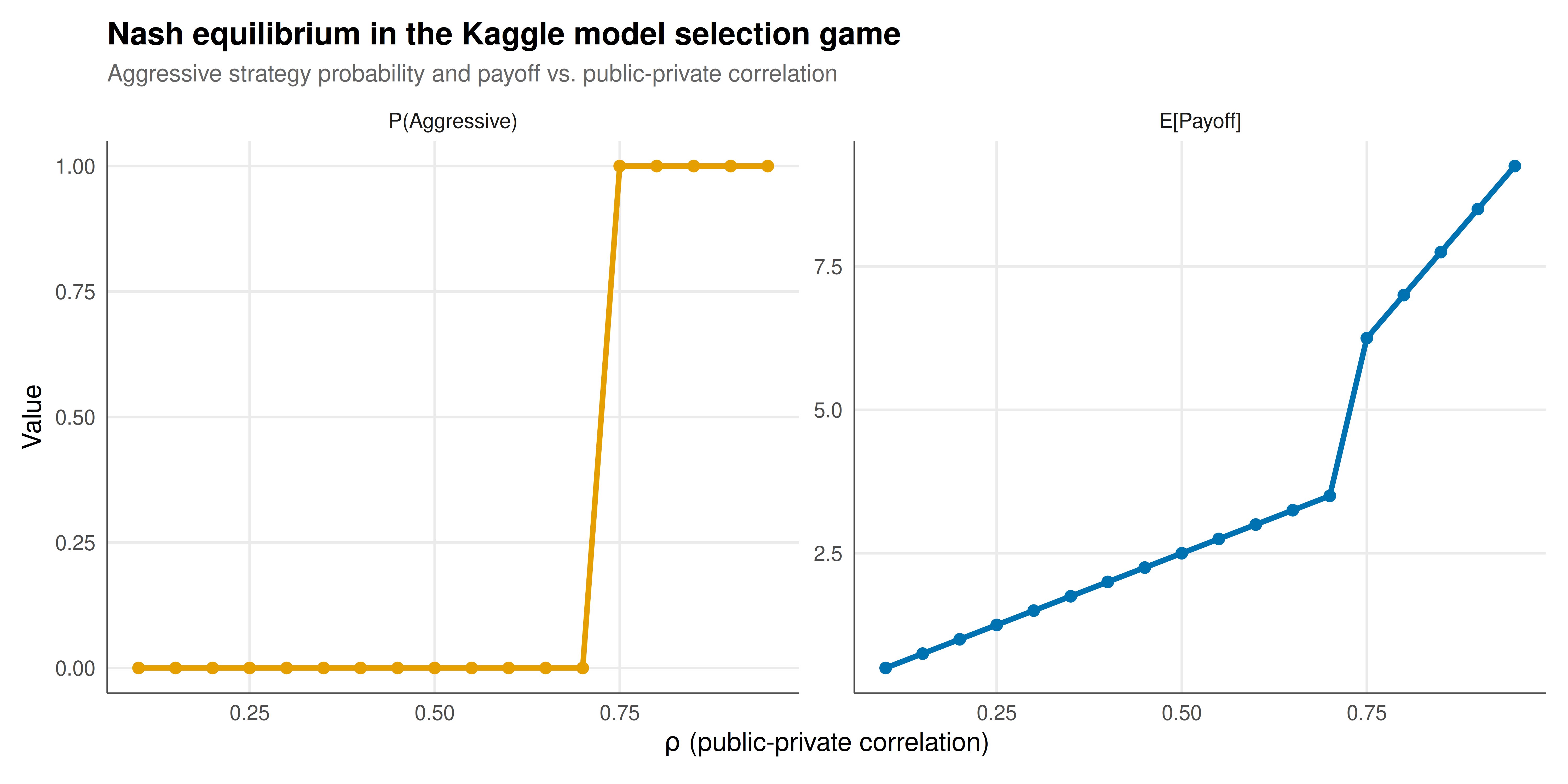
The figure shows how Nash equilibrium mixing probability and expected payoff change as a function of the public-private score correlation.

plot_data <- results %>%
  pivot_longer(cols = c(p_aggressive, eq_payoff),
               names_to = "metric", values_to = "value") %>%
  mutate(metric = factor(metric,
                         levels = c("p_aggressive", "eq_payoff"),
                         labels = c("P(Aggressive)", "E[Payoff]")))

p_static <- ggplot(plot_data, aes(x = rho, y = value, color = metric)) +
  geom_line(linewidth = 1.2) +
  geom_point(size = 2) +
  facet_wrap(~ metric, scales = "free_y") +
  scale_color_manual(values = okabe_ito[c(1, 5)]) +
  labs(title = "Nash equilibrium in the Kaggle model selection game",
       subtitle = "Aggressive strategy probability and payoff vs. public-private correlation",
       x = expression(rho ~ "(public-private correlation)"),
       y = "Value") +
  theme_publication() +
  theme(legend.position = "none")

p_static

Figure 1: Nash equilibrium analysis of the Kaggle model selection game. Left panel: probability of choosing the aggressive (high-variance) model at equilibrium as a function of public-private score correlation. Right panel: corresponding equilibrium expected payoff. Higher correlation favors aggressive strategies since public leaderboard signal is reliable. Parameters: prize v = 10, overfitting penalty c = 5. Okabe-Ito palette.

Interactive figure

The interactive version lets users hover over data points to inspect exact Nash equilibrium values at each correlation level alongside the payoff matrix entries.

p_int <- ggplot(results,
                aes(x = rho, y = p_aggressive,
                    text = paste0("Correlation: ", round(rho, 2),
                                  "\nP(Aggressive): ", round(p_aggressive, 3),
                                  "\nE[Payoff]: ", round(eq_payoff, 2),
                                  "\nU(A,A): ", round(u_AA, 2),
                                  "\nU(C,C): ", round(u_CC, 2)))) +
  geom_line(color = okabe_ito[1], linewidth = 1) +
  geom_point(aes(size = eq_payoff), color = okabe_ito[5], alpha = 0.7) +
  scale_size_continuous(name = "E[Payoff]", range = c(2, 6)) +
  labs(title = "Nash equilibrium: aggressive model probability",
       x = "Public-private correlation", y = "P(Aggressive)") +
  theme_publication()

ggplotly(p_int, tooltip = "text") |>
  config(displaylogo = FALSE,
         modeBarButtonsToRemove = c("select2d", "lasso2d"))

Figure 2

Interpretation

The Nash equilibrium analysis reveals a clear and intuitive pattern: as the correlation between public and private test sets increases, competitors rationally shift toward more aggressive modeling strategies. When \(\rho = 0.3\), the public leaderboard is a weak signal, and the equilibrium heavily favors conservative models. The probability of choosing the aggressive strategy is low because the expected overfitting penalty dominates the potential gain from a high public score. In this regime, experienced Kagglers follow the well-known advice to “trust your local cross-validation.” Conversely, when \(\rho = 0.9\), the public leaderboard is highly informative, and aggressive strategies become rational because models that score well publicly are very likely to score well privately.

The leaderboard shakeup simulation quantifies this effect from a different angle. At low correlation (\(\rho = 0.3\)), the mean rank correlation between public and private leaderboards is modest, confirming that dramatic shakeups are expected. The standard deviation of rank correlations is also substantial, meaning that outcomes are highly unpredictable. This unpredictability is precisely what makes the low-correlation regime strategically interesting: competitors face genuine uncertainty about whether their public ranking will hold. At \(\rho = 0.9\), rank correlations are consistently high, and shakeups are rare.

The game-theoretic framework explains several empirically observed phenomena in Kaggle competitions. First, the prevalence of ensemble methods (stacking, blending) can be understood as variance reduction – a way to shift from the aggressive to the conservative region of the strategy space without sacrificing expected accuracy. Teams that build diverse model ensembles are effectively playing the conservative strategy while maintaining competitive point estimates. Second, the practice of “leaderboard probing” – submitting known outputs to extract information about the test set – is rational only when the information gain exceeds the leakage cost \(\lambda\). In competitions with many participants, the leakage cost is effectively zero (your score is just one among thousands), which explains why probing is widespread in large competitions but riskier in small ones.

The model also illuminates why Kaggle’s rule limiting daily submissions is a well-designed mechanism. Without this constraint, the game degenerates: the dominant strategy becomes exhaustive probing, which eliminates the distinction between public and private leaderboards. The submission limit acts as a budget constraint that forces competitors to be strategic about when and what they submit. From a mechanism design perspective, this is analogous to a bid limit in an auction – it shapes the strategy space to produce more desirable equilibrium behavior.

A limitation of our two-strategy model is that real competitors choose from a continuum of model complexities, not a binary aggressive-conservative split. Extending the model to continuous strategy spaces would allow analysis of interior equilibria and comparative statics on parameters such as team size, competition duration, and prize distribution. Nevertheless, the binary model captures the essential strategic tension and provides actionable insights for competition participants.

Extensions & related tutorials

This strategic analysis of competitions connects to broader game-theoretic concepts explored elsewhere on the site.

• Fictitious play convergence
• No-regret learning in games
• World Bank development games
• Matrix games and linear algebra
• Deep reinforcement learning for strategic games

References