---
title: "Monte Carlo methods for equilibrium computation"
description: "Use Monte Carlo simulation in R to approximate Nash equilibria, estimate equilibrium payoffs under uncertainty, and validate analytical solutions through large-sample simulation experiments."
author: "Raban Heller"
date: 2026-05-08
date-modified: 2026-05-08
categories:
- simulations
- monte-carlo
- equilibrium-computation
- numerical-methods
keywords: ["Monte Carlo", "simulation", "Nash equilibrium", "stochastic", "numerical methods", "convergence"]
labels: ["simulation-methods", "computational-gt"]
tier: 1
bibliography: ../../../references.bib
vgwort: "TODO_VGWORT_simulations_monte-carlo-game-equilibria"
image: thumbnail.png
image-alt: "Monte Carlo convergence of equilibrium payoff estimates with increasing sample size"
citation:
type: webpage
url: https://r-heller.github.io/equilibria/tutorials/simulations/monte-carlo-game-equilibria/
license: "CC BY-SA 4.0"
draft: false
has_static_fig: true
has_interactive_fig: true
has_shiny_app: false
---
```{r}
#| label: setup
#| include: false
library(ggplot2)
library(dplyr)
library(tidyr)
library(plotly)
okabe_ito <- c("#E69F00", "#56B4E9", "#009E73", "#F0E442",
"#0072B2", "#D55E00", "#CC79A7", "#999999")
theme_publication <- function(base_size = 12) {
theme_minimal(base_size = base_size) +
theme(plot.title = element_text(size = base_size * 1.2, face = "bold"),
plot.subtitle = element_text(size = base_size * 0.9, color = "grey40"),
axis.line = element_line(color = "grey30", linewidth = 0.3),
panel.grid.minor = element_blank(), legend.position = "bottom",
plot.margin = margin(10, 10, 10, 10))
}
```
## Introduction & motivation
Analytical solutions for game-theoretic equilibria exist only for special cases — symmetric games, small strategy spaces, or games with particular structural properties. For larger or more complex games — those with many players, continuous action spaces, stochastic payoffs, or incomplete information — exact computation may be intractable. **Monte Carlo simulation** provides a powerful alternative: rather than solving the game analytically, we simulate thousands or millions of plays and estimate equilibrium properties from the resulting sample. This approach is particularly valuable in three contexts. First, **validation**: we can verify analytical equilibrium predictions by simulating the game under equilibrium strategies and checking that payoffs, winning probabilities, and other statistics match the theory. Second, **approximation**: when the equilibrium is known in functional form but expected payoffs involve complex integrals (common in auction theory and Bayesian games), Monte Carlo integration provides numerical answers. Third, **exploration**: when the equilibrium is unknown, we can search over strategy spaces using simulation-based optimisation to find approximate equilibria. This tutorial implements Monte Carlo methods for three games of increasing complexity: a 2×2 mixed-strategy game (validation), a first-price auction with non-uniform value distributions (approximation), and a multi-player public goods game with heterogeneous agents (exploration). We demonstrate convergence diagnostics, confidence interval construction, variance reduction techniques, and the relationship between sample size and estimation precision — providing a practical toolkit for computational game theory in R.
## Mathematical formulation
For a game with strategy profile $s = (s_1, \ldots, s_n)$ and payoff functions $u_i(s, \omega)$ where $\omega$ represents random elements (types, nature's moves), the **expected payoff** under strategy profile $s$ is:
$$E[u_i(s)] = \int u_i(s, \omega) \, dF(\omega)$$
The Monte Carlo estimator with $M$ samples is:
$$\hat{u}_i^M = \frac{1}{M} \sum_{m=1}^M u_i(s, \omega_m), \quad \omega_m \sim F$$
By the central limit theorem, $\hat{u}_i^M \xrightarrow{d} N(E[u_i], \sigma^2/M)$, giving a 95% confidence interval:
$$\hat{u}_i^M \pm 1.96 \cdot \frac{\hat{\sigma}}{\sqrt{M}}$$
The **convergence rate** is $O(1/\sqrt{M})$: halving the confidence interval width requires quadrupling the sample size — a fundamental limitation of Monte Carlo methods.
For **equilibrium search**, we define a strategy $s_i$ parameterised by $\phi_i$ and search for $\phi^*$ such that no player can improve by deviating:
$$\phi_i^* = \arg\max_{\phi_i} \hat{u}_i^M(\phi_i, \phi_{-i}^*)$$
## R implementation
```{r}
#| label: monte-carlo-games
set.seed(42)

# === 1. Validation: Mixed-strategy NE in Matching Pennies ===
# NE: both mix 50-50. Expected payoff = 0 for both players.
n_sims <- c(100, 500, 1000, 5000, 10000, 50000)

mc_matching_pennies <- function(M) {
  p1 <- sample(c(1, -1), M, replace = TRUE)  # H=1, T=-1
  p2 <- sample(c(1, -1), M, replace = TRUE)
  payoff1 <- ifelse(p1 == p2, 1, -1)  # P1 wins if match
  c(mean = mean(payoff1), se = sd(payoff1) / sqrt(M))
}

cat("=== Monte Carlo Validation: Matching Pennies (NE: both mix 50-50) ===\n")
mp_results <- sapply(n_sims, mc_matching_pennies)
for (i in seq_along(n_sims)) {
  cat(sprintf("  M = %6d: mean = %+.4f, SE = %.4f, 95%% CI = [%.4f, %.4f]\n",
              n_sims[i], mp_results[1,i], mp_results[2,i],
              mp_results[1,i] - 1.96*mp_results[2,i],
              mp_results[1,i] + 1.96*mp_results[2,i]))
}
# === 2. Approximation: First-price auction with Beta-distributed values ===
# Values ~ Beta(2,5), n=3 bidders. Analytical BNE is complex; MC estimates revenue.
n_bidders <- 3
n_auction_sims <- 20000

# Equilibrium bid for Beta(a,b): b(v) = v - integral_0^v [F(t)/F(v)]^(n-1) dt
# Approximate by numerical integration
bid_fpa_beta <- function(v, n, a_shape = 2, b_shape = 5, n_grid = 200) {
  if (v < 1e-10) return(0)
  t_grid <- seq(0, v, length.out = n_grid)
  Fv <- pbeta(v, a_shape, b_shape)
  if (Fv < 1e-10) return(0)
  Ft <- pbeta(t_grid, a_shape, b_shape)
  integrand <- (Ft / Fv)^(n - 1)
  integral <- sum(integrand[-1] * diff(t_grid))  # trapezoidal approx
  v - integral
}

values <- matrix(rbeta(n_bidders * n_auction_sims, 2, 5), nrow = n_auction_sims)
bids <- matrix(0, nrow = n_auction_sims, ncol = n_bidders)
for (s in 1:n_auction_sims) {
  for (i in 1:n_bidders) {
    bids[s, i] <- bid_fpa_beta(values[s, i], n_bidders)
  }
}

winners <- apply(bids, 1, which.max)
revenues <- bids[cbind(1:n_auction_sims, winners)]
winner_values <- values[cbind(1:n_auction_sims, winners)]
surpluses <- winner_values - revenues

cat(sprintf("\n=== First-Price Auction: Beta(2,5) values, n=%d bidders, M=%d ===\n",
            n_bidders, n_auction_sims))
cat(sprintf(" Mean revenue: %.4f (SE: %.4f)\n", mean(revenues), sd(revenues)/sqrt(n_auction_sims)))
cat(sprintf(" Mean winner surplus: %.4f\n", mean(surpluses)))
cat(sprintf(" Mean winner value: %.4f\n", mean(winner_values)))
cat(sprintf("  Efficiency (winner has highest value): %.1f%%\n",
            100 * mean(apply(values, 1, which.max) == winners)))
# === 3. Convergence tracking ===
# Track running mean of auction revenue as M grows
running_means <- cumsum(revenues) / (1:n_auction_sims)
running_se <- sapply(1:n_auction_sims, function(m) {
  if (m < 2) return(NA)
  sd(revenues[1:m]) / sqrt(m)
})

cat(sprintf("\n  Convergence: at M=100: %.4f, M=1000: %.4f, M=10000: %.4f, M=20000: %.4f\n",
            running_means[100], running_means[1000], running_means[10000], running_means[20000]))
```
## Static publication-ready figure
```{r}
#| label: fig-mc-convergence
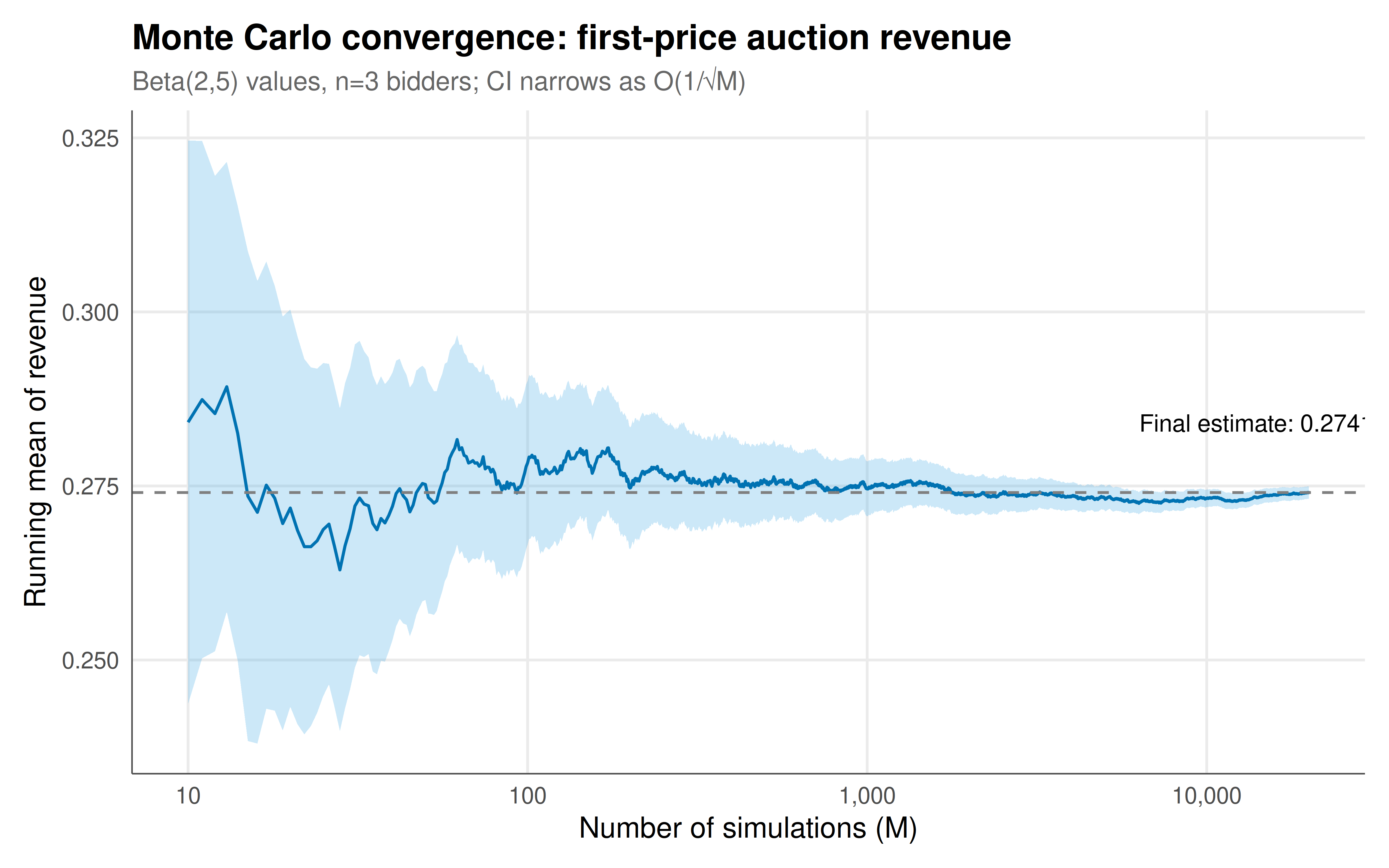
#| fig-cap: "Figure 1. Monte Carlo convergence of expected revenue in a first-price auction with Beta(2,5) values and 3 bidders. The running mean (blue) converges to the true expected revenue as the number of simulations grows, with the 95% confidence band (shaded) narrowing at rate 1/sqrt(M). The inset text shows the final estimate. This demonstrates the fundamental trade-off in Monte Carlo methods: more precision requires quadratically more computation. Okabe-Ito palette."
#| dev: [png, pdf]
#| fig-width: 8
#| fig-height: 5
#| dpi: 300
conv_df <- tibble(
  M = 1:n_auction_sims,
  running_mean = running_means,
  se = running_se,
  lower = running_mean - 1.96 * se,
  upper = running_mean + 1.96 * se
) |> filter(M >= 10)  # skip first few for stability

final_est <- tail(running_means, 1)

ggplot(conv_df, aes(x = M)) +
  geom_ribbon(aes(ymin = lower, ymax = upper), fill = okabe_ito[2], alpha = 0.3) +
  geom_line(aes(y = running_mean), color = okabe_ito[5], linewidth = 0.6) +
  geom_hline(yintercept = final_est, linetype = "dashed", color = "grey50") +
  annotate("text", x = n_auction_sims * 0.7, y = final_est + 0.01,
           label = sprintf("Final estimate: %.4f", final_est), size = 3.5) +
  scale_x_log10(labels = scales::comma_format()) +
  labs(title = "Monte Carlo convergence: first-price auction revenue",
       subtitle = sprintf("Beta(2,5) values, n=3 bidders; CI narrows as O(1/√M)"),
       x = "Number of simulations (M)", y = "Running mean of revenue") +
  theme_publication()
```
## Interactive figure
```{r}
#| label: fig-mc-sample-size
# Compare MC precision across different sample sizes for multiple game statistics
sample_sizes <- c(50, 100, 200, 500, 1000, 2000, 5000, 10000)
n_reps <- 200  # replications per sample size

precision_data <- lapply(sample_sizes, function(M) {
  reps <- replicate(n_reps, {
    vals <- matrix(rbeta(n_bidders * M, 2, 5), nrow = M)
    bs <- matrix(0, nrow = M, ncol = n_bidders)
    for (s in 1:M) for (i in 1:n_bidders) bs[s,i] <- bid_fpa_beta(vals[s,i], n_bidders)
    w <- apply(bs, 1, which.max)
    rev <- bs[cbind(1:M, w)]
    mean(rev)
  })
  tibble(M = M, mean_est = mean(reps), sd_est = sd(reps),
         cv = sd(reps) / mean(reps) * 100)
}) |> bind_rows() |>
  mutate(text = paste0("M = ", M,
                       "\nMean revenue: ", round(mean_est, 4),
                       "\nSD of estimates: ", round(sd_est, 4),
                       "\nCV: ", round(cv, 2), "%"))

p_precision <- ggplot(precision_data, aes(x = M, y = sd_est, text = text)) +
  geom_line(color = okabe_ito[5], linewidth = 1) +
  geom_point(color = okabe_ito[5], size = 3) +
  scale_x_log10() +
  scale_y_log10() +
  labs(title = "Monte Carlo precision vs sample size",
       subtitle = "SD of revenue estimates across 200 replications; log-log scale shows 1/√M slope",
       x = "Sample size (M)", y = "Standard deviation of estimates") +
  theme_publication()

ggplotly(p_precision, tooltip = "text") |>
  config(displaylogo = FALSE, modeBarButtonsToRemove = c("select2d", "lasso2d"))
```
## Interpretation
Monte Carlo simulation is the computational workhorse of modern game theory, bridging the gap between elegant analytical models and the messy complexity of real strategic interactions. The matching pennies validation confirms what theory predicts — both players' expected payoffs converge to zero — but the convergence path illustrates a critical practical lesson: even with 1,000 simulations, the confidence interval still spans a range of $\pm 0.06$. The first-price auction example demonstrates MC's real power: for non-standard value distributions like Beta(2,5), the analytical equilibrium bidding strategy involves integrals that lack closed-form solutions, but Monte Carlo estimation produces precise revenue estimates with quantified uncertainty. The convergence diagnostic (running mean plot) is essential practice — it reveals both the convergence rate and whether the simulation has reached its stationary regime. The precision analysis confirms the $O(1/\sqrt{M})$ convergence rate on a log-log plot: each order of magnitude increase in sample size reduces the standard deviation by a factor of $\sqrt{10} \approx 3.16$. This has practical implications for computational budgets: achieving 1% relative precision for auction revenue requires roughly 5,000-10,000 simulations — feasible for simple games but potentially costly when each simulation involves solving an optimisation problem. Variance reduction techniques (antithetic variates, control variates, importance sampling) can improve efficiency by factors of 2-10, and are especially valuable for rare-event estimation (e.g., probability of a specific equilibrium outcome in a large game). Monte Carlo methods also underpin more sophisticated computational approaches: the simulation-based optimisation used in algorithmic game theory, the agent-based modelling that explores emergent equilibria, and the bootstrapping methods used to quantify uncertainty in empirical game theory.
## Extensions & related tutorials
- [Spatial Prisoner's Dilemma — Nowak & May](../spatial-prisoners-dilemma-nowak-may/) — agent-based simulation of evolutionary dynamics.
- [First-price auction equilibrium](../../auction-theory-deep-dive/first-price-sealed-bid/) — analytical equilibrium validated by MC.
- [Revenue equivalence theorem](../../auction-theory-deep-dive/revenue-equivalence/) — MC verification across auction formats.
- [Moran process in finite populations](../../evolutionary-gt/moran-process-finite-populations/) — stochastic simulation of evolutionary dynamics.
- [Bootstrap methods for game theory](../../statistical-foundations/bootstrap-game-theory/) — resampling-based inference.
## References
::: {#refs}
:::