---
title: "All-pay auctions and the economics of lobbying"
description: "Analyse the all-pay auction in R where all bidders pay their bids regardless of winning, derive the symmetric equilibrium with uniform values, and apply the model to lobbying, rent-seeking, and political campaigns."
author: "Raban Heller"
date: 2026-05-08
date-modified: 2026-05-08
categories:
- auction-theory-deep-dive
- all-pay-auction
- lobbying
- rent-seeking
keywords: ["all-pay auction", "lobbying", "rent-seeking", "Tullock contest", "political competition", "bid shading"]
labels: ["auction-theory", "political-economy"]
tier: 1
bibliography: ../../../references.bib
vgwort: "TODO_VGWORT_auction-theory-deep-dive_all-pay-auction-lobbying"
image: thumbnail.png
image-alt: "Equilibrium bidding strategies in all-pay auctions compared to first-price auctions"
citation:
type: webpage
url: https://r-heller.github.io/equilibria/tutorials/auction-theory-deep-dive/all-pay-auction-lobbying/
license: "CC BY-SA 4.0"
draft: false
has_static_fig: true
has_interactive_fig: true
has_shiny_app: false
---
```{r}
#| label: setup
#| include: false
library(ggplot2)
library(dplyr)
library(tidyr)
library(plotly)
okabe_ito <- c("#E69F00", "#56B4E9", "#009E73", "#F0E442",
"#0072B2", "#D55E00", "#CC79A7", "#999999")
theme_publication <- function(base_size = 12) {
theme_minimal(base_size = base_size) +
theme(plot.title = element_text(size = base_size * 1.2, face = "bold"),
plot.subtitle = element_text(size = base_size * 0.9, color = "grey40"),
axis.line = element_line(color = "grey30", linewidth = 0.3),
panel.grid.minor = element_blank(), legend.position = "bottom",
plot.margin = margin(10, 10, 10, 10))
}
```
## Introduction & motivation
In most auctions, only the winner pays. But in many real-world contests, **all participants pay** regardless of whether they win. Lobbying is the canonical example: firms spend millions on lobbying efforts, and every firm pays its lobbyists whether or not the favourable regulation is obtained. Political campaigns spend on advertising and voter mobilisation — the losing candidate's expenditures are sunk. Patent races, R&D competitions, litigation, and military conflicts all share this "all-pay" structure: resources committed to the contest are irreversibly spent. The **all-pay auction** formalises these situations: $n$ bidders submit bids, the highest bidder wins a prize of value $V$, and every bidder pays their own bid regardless of outcome. The equilibrium is strikingly different from standard auctions. With $n$ bidders and values $v_i \sim U[0,1]$, the symmetric equilibrium bid function is $b^*(v) = \frac{n-1}{n} v^n$ — bidders shade much more aggressively than in first-price auctions ($b^*_{FP} = \frac{n-1}{n}v$) because every bid is paid, making aggressive bidding extremely costly. A key result from the theory of contests is **complete rent dissipation**: in equilibrium, total expected expenditure by all bidders equals the prize value, so the social surplus from the contest is zero — all rents are consumed by the competition itself. This connects to Gordon Tullock's rent-seeking literature: when firms compete for government-granted monopoly rights, the wasteful lobbying expenditures can consume the entire monopoly profit, making the rent-seeking game socially costly even when a monopoly is granted. This tutorial derives the all-pay equilibrium, compares it with first-price auctions, simulates rent dissipation, and applies the model to lobbying with asymmetric contestants.
## Mathematical formulation
**All-pay auction** with $n$ bidders, values $v_i \sim U[0,1]$ independently. All bidders pay their bids; highest bidder wins prize $V = 1$.
**Symmetric BNE**: The equilibrium bid function is:
$$b^*(v) = \frac{n-1}{n} v^n$$
*Derivation*: Bidder with value $v$ maximises $(v - 0) \cdot P(\text{win}) - b = v \cdot F_{\max}(b^{-1}(b))^{n-1} - b$ where $F_{\max}$ is the CDF of the highest competing value. With $b^{-1}(b) = (nb/(n-1))^{1/n}$, the FOC gives $b^*(v) = \frac{n-1}{n}v^n$.
**Expected revenue** (= total expenditure by all bidders): $E[R] = n \cdot E[b^*(v)] = n \cdot \frac{n-1}{n} \cdot \frac{1}{n+1} = \frac{n-1}{n+1}$
This equals the expected revenue of the first-price and second-price auctions — **revenue equivalence** holds.
**Tullock contest** (imperfectly discriminating): Player $i$ with effort $x_i$ wins with probability $p_i = x_i^r / \sum_j x_j^r$ where $r$ is the "decisiveness" parameter. The all-pay auction is the limit $r \to \infty$.
## R implementation
```{r}
#| label: all-pay-auction
set.seed(42)

# === Equilibrium bidding ===
bid_allpay <- function(v, n) ((n - 1) / n) * v^n
bid_firstprice <- function(v, n) ((n - 1) / n) * v

cat("=== All-Pay Auction vs First-Price Auction ===\n\n")
# Compare bid functions
cat("--- Bid functions at v = 0.5, 0.8, 1.0 ---\n")
for (v in c(0.5, 0.8, 1.0)) {
  for (n in c(2, 5, 10)) {
    cat(sprintf("  v=%.1f, n=%2d: all-pay b=%.4f, FPA b=%.4f, ratio=%.3f\n",
                v, n, bid_allpay(v, n), bid_firstprice(v, n),
                bid_allpay(v, n) / bid_firstprice(v, n)))
  }
}
# === Simulate and verify revenue equivalence ===
n_sims <- 20000
sim_results <- lapply(c(2, 3, 5, 10), function(n) {
  values <- matrix(runif(n * n_sims), nrow = n_sims)

  # All-pay: everyone pays
  bids_ap <- bid_allpay(values, n)
  rev_ap <- rowSums(bids_ap)  # total expenditure

  # First-price: only winner pays
  bids_fp <- bid_firstprice(values, n)
  winners_fp <- apply(bids_fp, 1, which.max)
  rev_fp <- bids_fp[cbind(1:n_sims, winners_fp)]

  tibble(n = n, rev_ap = mean(rev_ap), rev_fp = mean(rev_fp),
         theoretical = (n - 1) / (n + 1),
         rent_dissipation = mean(rev_ap) / 1.0)  # prize = 1
}) |> bind_rows()

cat("\n--- Revenue Equivalence Verification ---\n")
cat(sprintf(" %-4s %-12s %-12s %-12s\n", "n", "All-pay", "First-price", "Theoretical"))
for (i in 1:nrow(sim_results)) {
  cat(sprintf("  %-4d %-12.4f %-12.4f %-12.4f\n",
              sim_results$n[i], sim_results$rev_ap[i],
              sim_results$rev_fp[i], sim_results$theoretical[i]))
}
# === Tullock contest ===
cat("\n--- Tullock Contest (2 symmetric players, V=1) ---\n")
# NE: x* = V*r/(4) for 2 players with linear cost
for (r in c(0.5, 1, 2, 5)) {
  x_star <- r / 4  # symmetric NE effort
  total_effort <- 2 * x_star
  cat(sprintf("  r = %.1f: x* = %.3f, total effort = %.3f, dissipation = %.0f%%\n",
              r, x_star, total_effort, 100 * total_effort))
}
cat(" (r → ∞ = all-pay auction: 100% dissipation)\n")
```
## Static publication-ready figure
```{r}
#| label: fig-allpay-bidding
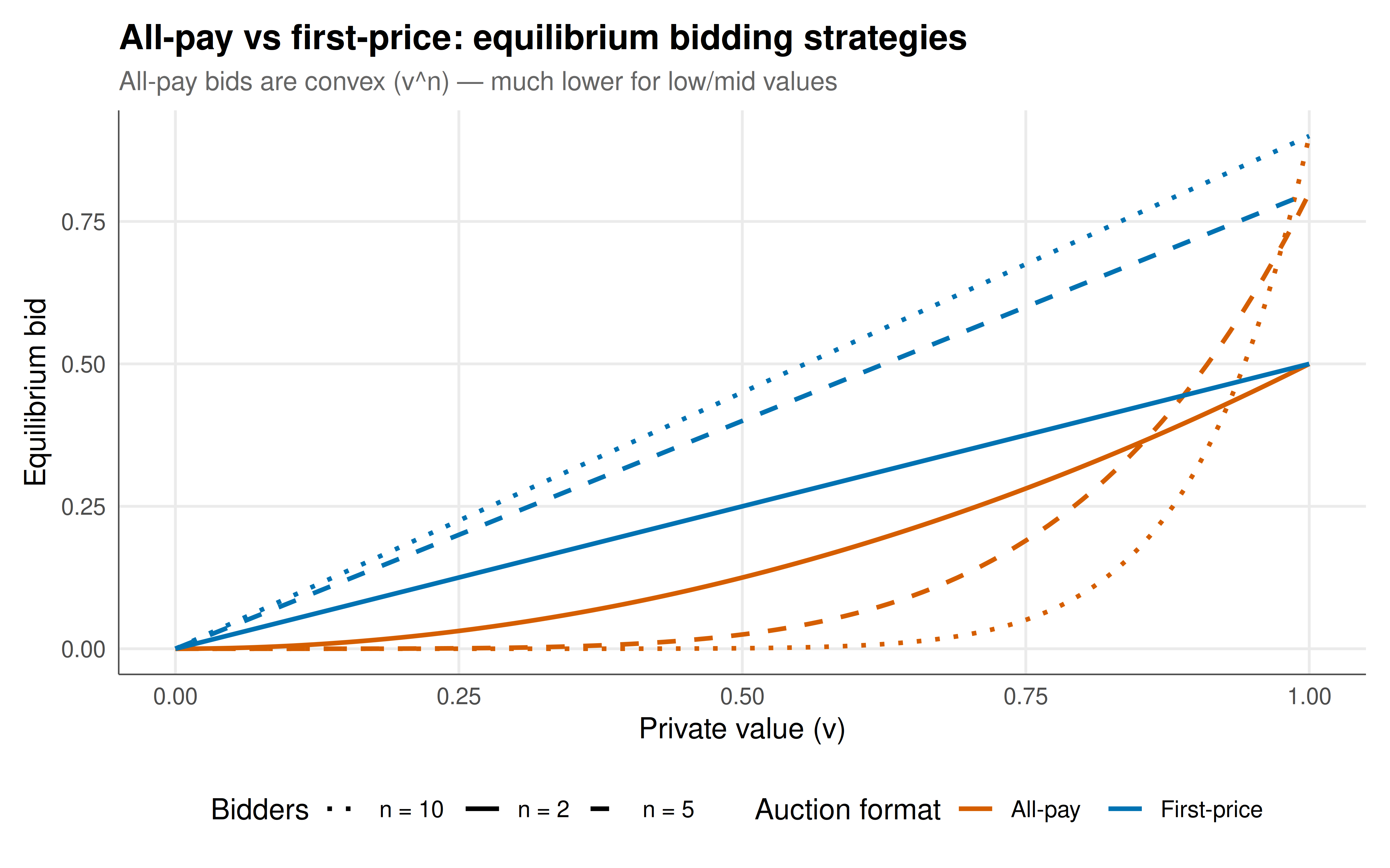
#| fig-cap: "Figure 1. Equilibrium bidding strategies: all-pay auction vs first-price auction for different numbers of bidders. All-pay bids are dramatically lower for most values because every bid is paid — bidders shade aggressively to limit losses. The gap narrows for high values where the probability of winning is large. With more bidders, both bid functions shift but the all-pay curve remains convex (v^n) while first-price remains linear. Okabe-Ito palette."
#| dev: [png, pdf]
#| fig-width: 8
#| fig-height: 5
#| dpi: 300
v_seq <- seq(0, 1, 0.01)
bid_df <- expand.grid(v = v_seq, n = c(2, 5, 10)) |>
  mutate(
    allpay = bid_allpay(v, n),
    firstprice = bid_firstprice(v, n),
    n_label = paste0("n = ", n)
  ) |>
  pivot_longer(c(allpay, firstprice), names_to = "format", values_to = "bid") |>
  mutate(format = ifelse(format == "allpay", "All-pay", "First-price"))

ggplot(bid_df, aes(x = v, y = bid, color = format, linetype = n_label)) +
  geom_line(linewidth = 0.9) +
  scale_color_manual(values = c("All-pay" = okabe_ito[6], "First-price" = okabe_ito[5]),
                      name = "Auction format") +
  scale_linetype_manual(values = c("n = 2" = "solid", "n = 5" = "dashed", "n = 10" = "dotted"),
                         name = "Bidders") +
  labs(title = "All-pay vs first-price: equilibrium bidding strategies",
       subtitle = "All-pay bids are convex (v^n) — much lower for low/mid values",
       x = "Private value (v)", y = "Equilibrium bid") +
  theme_publication()
```
## Interactive figure
```{r}
#| label: fig-allpay-dissipation
# Rent dissipation across number of bidders
n_seq <- 2:20
dissipation_df <- tibble(
  n = n_seq,
  total_expenditure = (n_seq - 1) / (n_seq + 1),
  winner_surplus = 1 / (n_seq * (n_seq + 1)),
  loser_loss = (n_seq - 1) / (n_seq * (n_seq + 1))
) |>
  pivot_longer(-n, names_to = "metric", values_to = "value") |>
  mutate(
    label = case_when(
      metric == "total_expenditure" ~ "Total expenditure (rent dissipation)",
      metric == "winner_surplus" ~ "Winner's expected surplus",
      metric == "loser_loss" ~ "Expected loss per loser"
    ),
    text = paste0("n = ", n, "\n", label, ": ", round(value, 4))
  )

p_diss <- ggplot(dissipation_df, aes(x = n, y = value, color = label, text = text)) +
  geom_line(linewidth = 1) +
  geom_point(size = 1.5) +
  scale_color_manual(values = okabe_ito[c(6, 3, 1)], name = NULL) +
  labs(title = "All-pay auction: rent dissipation increases with competition",
       subtitle = "Total expenditure → 1 (= prize value); winner surplus → 0",
       x = "Number of bidders", y = "Expected value") +
  theme_publication()

ggplotly(p_diss, tooltip = "text") |>
  config(displaylogo = FALSE, modeBarButtonsToRemove = c("select2d", "lasso2d"))
```
## Interpretation
The all-pay auction provides the game-theoretic foundation for understanding wasteful competition. When all contestants must pay regardless of outcome, the equilibrium involves aggressive bid shading (the convex $v^n$ bid function) that limits each individual's exposure, but collectively, total expenditure still equals the prize value — rent dissipation is complete. This result explains several puzzling real-world phenomena: why lobbying expenditures in Washington often approach the value of the regulation being sought; why political campaign spending seems "excessive" relative to the value of office; and why patent races can consume most of the expected patent value in R&D costs. The comparison with first-price auctions is illuminating: at $v = 0.5$ with 5 bidders, the first-price bid is 0.40 while the all-pay bid is only 0.025 — a factor of 16 lower. This extreme shading reflects the asymmetric risk: in an all-pay auction, bidding aggressively with a mediocre value is doubly costly (you probably lose AND you pay), while in a first-price auction you only pay if you win. The Tullock contest model shows how the "decisiveness" parameter $r$ controls the intensity of competition: at $r = 1$ (standard contest success function), total effort is only 50% of the prize; at $r = 2$, it reaches 100%; and as $r \to \infty$ (all-pay auction), all rents are dissipated. Policy implications are direct: reducing the decisiveness of contests (e.g., using lotteries instead of winner-take-all for government grants) can reduce wasteful rent-seeking while still selecting above-average contestants.
## Extensions & related tutorials
- [First-price sealed-bid auction](../first-price-sealed-bid/) — the standard where only winners pay.
- [Revenue equivalence theorem](../revenue-equivalence/) — why all four standard formats yield equal revenue.
- [War of attrition](../../evolutionary-gt/hawk-dove-war-of-attrition/) — continuous-time all-pay contest.
- [Colonel Blotto game](../../classical-games/colonel-blotto/) — multi-battlefield resource allocation.
- [Tragedy of the commons](../../case-studies/tragedy-of-the-commons/) — another model of wasteful competition.
## References
::: {#refs}
:::