Matching Pennies — the simplest zero-sum game

Analyse Matching Pennies as the canonical two-player zero-sum game with a unique mixed-strategy Nash equilibrium, implementing minimax strategies and expected payoff calculations in R.

Keywords

Matching Pennies, zero-sum, mixed strategy, minimax, randomization

Introduction & motivation

Matching Pennies is the simplest non-trivial zero-sum game: two players simultaneously choose Heads or Tails. Player 1 (the Matcher) wins if both coins match; Player 2 (the Mismatcher) wins if they differ. There is no pure-strategy Nash equilibrium — any pure strategy can be exploited by the opponent. The unique equilibrium requires both players to randomise uniformly: play Heads with probability 1/2. This game captures the essence of strategic uncertainty in competitive settings: penalty kicks in football, audit timing in tax enforcement, randomised inspection schedules, and any situation where predictability is punished. Matching Pennies is the 2×2 instance of the minimax theorem — the game value is 0, and both players can guarantee exactly 0 in expectation by mixing uniformly. Understanding this game deeply — why no pure equilibrium exists, why the mixed equilibrium is unique, and what the equilibrium mixing probability means operationally — provides the intuitive foundation for minimax theory, randomised strategies, and the interpretation of mixed Nash equilibria more broadly.

Mathematical formulation

\[ \begin{array}{c|cc} & H & T \\ \hline H & 1, -1 & -1, 1 \\ T & -1, 1 & 1, -1 \end{array} \]

This is a zero-sum game (\(u_1 + u_2 = 0\) in every cell). No pure NE exists: for any pure profile, the losing player can profitably deviate.

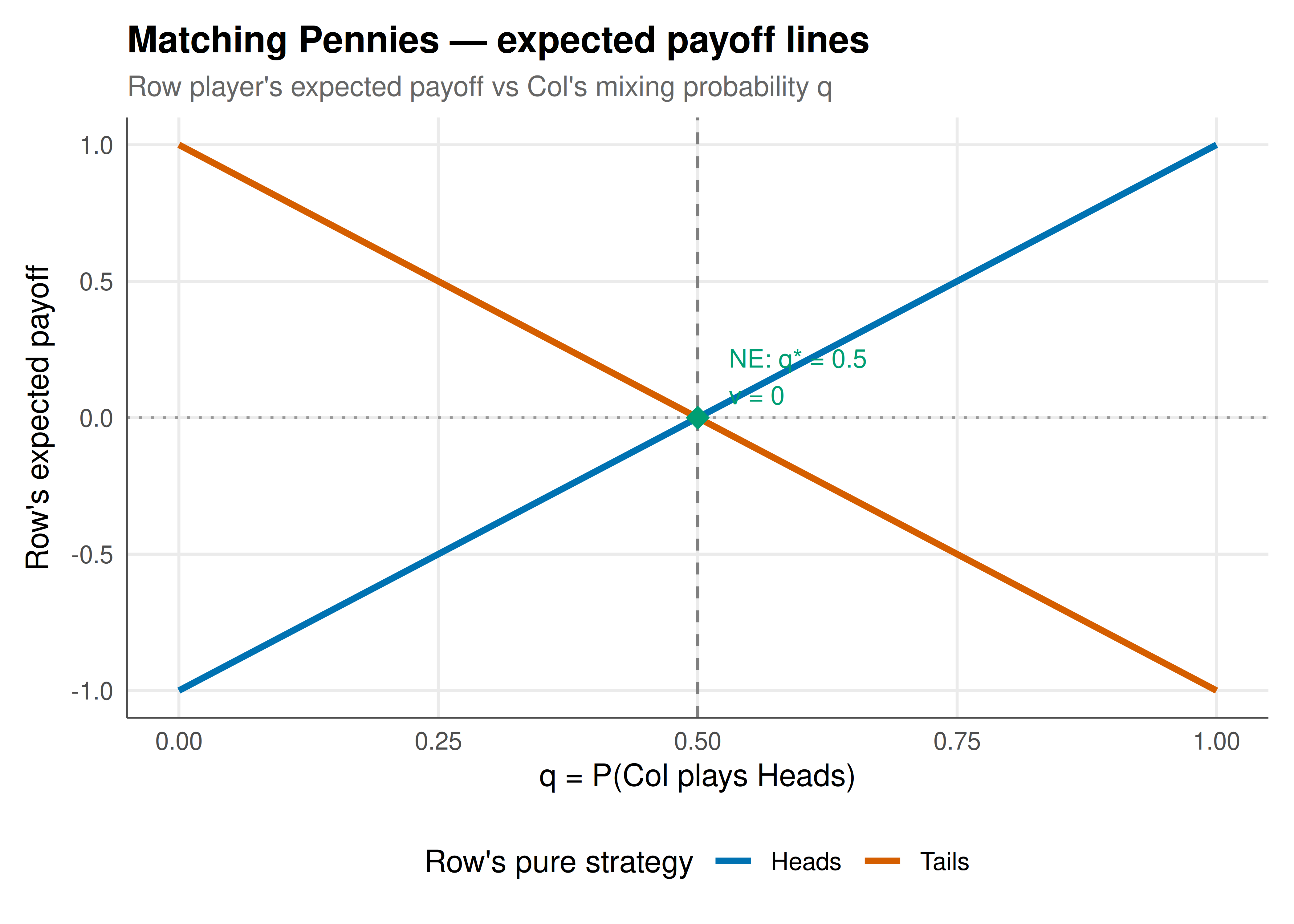
Mixed NE: Let \(p = P(\text{Row plays H})\) and \(q = P(\text{Col plays H})\). Row’s expected payoff from H: \(q \cdot 1 + (1-q)(-1) = 2q - 1\). Row’s expected payoff from T: \(q(-1) + (1-q)(1) = 1 - 2q\). Indifference requires \(2q - 1 = 1 - 2q\), giving \(q^* = 1/2\). By symmetry, \(p^* = 1/2\).

The game value is \(v = 0\): fair game under optimal play.

R implementation

# Matching Pennies payoff matrix
A_mp <- matrix(c(1, -1, -1, 1), nrow = 2,
               dimnames = list(c("H","T"), c("H","T")))

# Expected payoff calculations
expected_payoff_row <- function(p, q) {
  p * q * 1 + p * (1-q) * (-1) + (1-p) * q * (-1) + (1-p) * (1-q) * 1
}

# Verify: at equilibrium (p=0.5, q=0.5)
cat("Equilibrium expected payoff:", expected_payoff_row(0.5, 0.5), "\n")

Equilibrium expected payoff: 0 

# Show exploitability of pure strategies
cat("\nExploitability of pure strategies:\n")

Exploitability of pure strategies:

cat(sprintf("  Row plays pure H: Col plays T, Row gets %d\n", A_mp["H","T"]))

  Row plays pure H: Col plays T, Row gets -1

cat(sprintf("  Row plays pure T: Col plays H, Row gets %d\n", A_mp["T","H"]))

  Row plays pure T: Col plays H, Row gets -1

cat(sprintf("  Row plays 50/50: regardless of Col, Row expects %.1f\n",
            expected_payoff_row(0.5, 0.5)))

  Row plays 50/50: regardless of Col, Row expects 0.0

# Simulation: what happens when one player deviates from equilibrium?
set.seed(42)
n_rounds <- 10000
results <- tibble(
  round = 1:n_rounds,
  row_plays_h = runif(n_rounds) < 0.5,  # Row plays equilibrium
  col_plays_h = runif(n_rounds) < 0.7   # Col deviates: 70% heads
) |>
  mutate(
    match = (row_plays_h == col_plays_h),
    row_payoff = ifelse(match, 1, -1),
    cumulative_avg = cumsum(row_payoff) / round
  )

cat(sprintf("\nSimulation (10K rounds, Row=50/50, Col=70%% H):\n"))

Simulation (10K rounds, Row=50/50, Col=70% H):

cat(sprintf("  Row's average payoff: %.3f (should be ~0 despite Col's deviation)\n",
            mean(results$row_payoff)))

  Row's average payoff: 0.001 (should be ~0 despite Col's deviation)

Static publication-ready figure

q_seq <- seq(0, 1, by = 0.01)
payoff_lines <- tibble(
  q = rep(q_seq, 2),
  strategy = rep(c("Heads", "Tails"), each = length(q_seq)),
  payoff = c(2 * q_seq - 1, 1 - 2 * q_seq)
)

p_lines <- ggplot(payoff_lines, aes(x = q, y = payoff, color = strategy)) +
  geom_line(linewidth = 1.2) +
  geom_hline(yintercept = 0, linetype = "dotted", color = "grey60") +
  geom_vline(xintercept = 0.5, linetype = "dashed", color = "grey50") +
  geom_point(aes(x = 0.5, y = 0), color = okabe_ito[3], size = 4, shape = 18,
             inherit.aes = FALSE) +
  annotate("text", x = 0.53, y = 0.15, label = "NE: q* = 0.5\nv = 0",
           size = 3.5, hjust = 0, color = okabe_ito[3]) +
  scale_color_manual(values = c(Heads = okabe_ito[5], Tails = okabe_ito[6]),
                      name = "Row's pure strategy") +
  labs(
    title = "Matching Pennies — expected payoff lines",
    subtitle = "Row player's expected payoff vs Col's mixing probability q",
    x = "q = P(Col plays Heads)", y = "Row's expected payoff"
  ) +
  theme_publication()

p_lines

Figure 1: Figure 1. Expected payoff for Row in Matching Pennies as a function of Col’s mixing probability q, for each of Row’s pure strategies. The lines cross at q = 0.5 — the unique point where Row is indifferent between H and T. At this point, any mixing by Row yields 0 in expectation. Deviating from 50/50 creates exploitability. Okabe-Ito palette.

Interactive figure

sim_plot_data <- results |>
  filter(round <= 2000) |>
  mutate(text = paste0("Round: ", round,
                       "\nCum avg: ", round(cumulative_avg, 3)))

p_sim <- ggplot(sim_plot_data, aes(x = round, y = cumulative_avg, text = text)) +
  geom_line(color = okabe_ito[5], linewidth = 0.5, alpha = 0.7) +
  geom_hline(yintercept = 0, linetype = "dashed", color = okabe_ito[3]) +
  labs(
    title = "Cumulative average payoff — Row plays equilibrium vs biased Col",
    subtitle = "Row plays 50/50; Col deviates to 70% Heads. Row's guarantee holds.",
    x = "Round", y = "Cumulative average payoff"
  ) +
  theme_publication()

ggplotly(p_sim, tooltip = "text") |>
  config(displaylogo = FALSE,
         modeBarButtonsToRemove = c("select2d", "lasso2d"))

Figure 2

Interpretation

Matching Pennies teaches three fundamental lessons. First, pure strategies are exploitable in competitive settings: any predictable choice gives the opponent an advantage, which is why randomisation is essential. Second, the mixed equilibrium is a guarantee, not a choice: playing 50/50 does not mean Row expects to win anything — it means Row ensures a payoff of 0 regardless of what Col does. The simulation confirms this: even when Col deviates to 70% Heads, Row’s average payoff converges to 0, not to a positive number. This is the minimax guarantee in action. Third, mixed equilibrium mixing probabilities are determined by the opponent’s indifference, not by one’s own preferences: Row mixes 50/50 not because Row is indifferent (Row is), but because that mix makes Col indifferent, and vice versa. This subtle point is often misunderstood: the equilibrium is a fixed point of best-response mappings, not an expression of randomised preference. In applications, Matching Pennies explains why penalty kickers in football mix their shot directions, why tax auditors randomise inspection schedules, and why military deception requires genuine unpredictability rather than a fixed deception plan.

Extensions & related tutorials

• Zero-sum games and the minimax theorem — the general framework containing Matching Pennies.
• Mixed-strategy Nash equilibrium in 2×2 games — computing mixed NE for general games.
• Battle of the Sexes — a non-zero-sum game with three equilibria.
• Penalty kicks as a game — empirical application of Matching Pennies.
• Blotto games — multi-dimensional competitive allocation.

References