---
title: "Epsilon-equilibrium and approximate Nash equilibria"
description: "Implement epsilon-Nash equilibrium in R, analyse when approximate solutions suffice for practical predictions, compute the epsilon required for various games, and connect to computational complexity of exact Nash equilibrium finding."
author: "Raban Heller"
date: 2026-05-08
date-modified: 2026-05-08
categories:
- foundations
- epsilon-equilibrium
- approximate-equilibrium
- computational-complexity
keywords: ["epsilon-equilibrium", "approximate Nash", "bounded rationality", "PPAD", "computational game theory"]
labels: ["equilibrium-concepts", "computational-gt"]
tier: 1
bibliography: ../../../references.bib
vgwort: "TODO_VGWORT_foundations_epsilon-equilibrium-approximate"
image: thumbnail.png
image-alt: "Epsilon-Nash equilibrium regions showing how the set of approximate equilibria expands as epsilon increases"
citation:
type: webpage
url: https://r-heller.github.io/equilibria/tutorials/foundations/epsilon-equilibrium-approximate/
license: "CC BY-SA 4.0"
draft: false
has_static_fig: true
has_interactive_fig: true
has_shiny_app: false
---
```{r}
#| label: setup
#| include: false
library(ggplot2)
library(dplyr)
library(tidyr)
library(plotly)
okabe_ito <- c("#E69F00", "#56B4E9", "#009E73", "#F0E442",
"#0072B2", "#D55E00", "#CC79A7", "#999999")
theme_publication <- function(base_size = 12) {
theme_minimal(base_size = base_size) +
theme(plot.title = element_text(size = base_size * 1.2, face = "bold"),
plot.subtitle = element_text(size = base_size * 0.9, color = "grey40"),
axis.line = element_line(color = "grey30", linewidth = 0.3),
panel.grid.minor = element_blank(), legend.position = "bottom",
plot.margin = margin(10, 10, 10, 10))
}
```
## Introduction & motivation
Nash equilibrium demands perfection: every player must play an exact best response to the others' strategies. But in practice, players are boundedly rational, payoffs are estimated with error, and computation is costly. An **epsilon-Nash equilibrium** relaxes the best-response requirement: no player can gain more than $\epsilon$ by deviating. This seemingly minor relaxation has profound implications for both theory and practice.
From a practical standpoint, epsilon-equilibrium acknowledges that small deviations from best-responding are inevitable in real strategic interactions. A firm that could increase profits by 0.01% by adjusting its price is unlikely to do so — the computational and attention costs exceed the gain. An experimental subject whose expected payoff from switching strategies is a few cents will not reliably switch. Epsilon-equilibrium captures the idea that "close enough" to best-responding is all we can expect from real agents, and provides a framework for asking: how close is close enough?
From a computational standpoint, epsilon-equilibrium is central to the theory of algorithmic game theory. Finding an exact Nash equilibrium in a bimatrix game is PPAD-complete — believed to require exponential time in the worst case. But finding an epsilon-Nash equilibrium with $\epsilon = O(1/\text{poly}(n))$ is potentially easier, and the Lipton-Markakis-Mehta algorithm shows that an epsilon-equilibrium with logarithmic-size support always exists. This connects the computational difficulty of equilibrium to the precision required: if we are willing to accept approximate solutions, the problem may become tractable.
The concept also bridges to learning dynamics: many natural learning algorithms (fictitious play, no-regret learning, replicator dynamics) converge to epsilon-equilibria but not necessarily to exact Nash equilibria. Understanding the epsilon-equilibrium structure of a game tells us what learning algorithms can achieve and how quickly. This tutorial implements epsilon-equilibrium computation, visualises the set of approximate equilibria as epsilon varies, and analyses the relationship between game structure and the "cost of approximation."
## Mathematical formulation
**Epsilon-Nash equilibrium**: A strategy profile $\sigma^*$ is an $\epsilon$-Nash equilibrium if for every player $i$ and every strategy $s_i$:
$$u_i(\sigma^*_i, \sigma^*_{-i}) \geq u_i(s_i, \sigma^*_{-i}) - \epsilon$$
**Epsilon-regret**: The regret of player $i$ at profile $\sigma$ is:
$$r_i(\sigma) = \max_{s_i} u_i(s_i, \sigma_{-i}) - u_i(\sigma_i, \sigma_{-i})$$
Profile $\sigma$ is an $\epsilon$-NE iff $\max_i r_i(\sigma) \leq \epsilon$.
**Properties**: (1) Every Nash equilibrium is a 0-NE. (2) The set of $\epsilon$-NE is monotone: if $\epsilon_1 < \epsilon_2$, then $\text{NE}_{\epsilon_1} \subseteq \text{NE}_{\epsilon_2}$. (3) Every game has an $\epsilon$-NE in pure strategies for sufficiently large $\epsilon$.
## R implementation
```{r}
#| label: epsilon-equilibrium
set.seed(42)

cat("=== Epsilon-Nash Equilibrium ===\n\n")
# === Compute epsilon-regret for a strategy profile ===
compute_regret <- function(A, B, p, q) {
  # p = P(Top) for row, q = P(Left) for col
  # Row player's payoffs
  eu_top <- A[1,1]*q + A[1,2]*(1-q)
  eu_bot <- A[2,1]*q + A[2,2]*(1-q)
  eu_row <- p*eu_top + (1-p)*eu_bot
  regret_row <- max(eu_top, eu_bot) - eu_row

  # Column player's payoffs
  eu_left <- B[1,1]*p + B[2,1]*(1-p)
  eu_right <- B[1,2]*p + B[2,2]*(1-p)
  eu_col <- q*eu_left + (1-q)*eu_right
  regret_col <- max(eu_left, eu_right) - eu_col

  c(row = regret_row, col = regret_col, max = max(regret_row, regret_col))
}

# === Game 1: Prisoner's Dilemma ===
A_pd <- matrix(c(3, 0, 5, 1), 2, 2)
B_pd <- matrix(c(3, 5, 0, 1), 2, 2)
cat("--- Prisoner's Dilemma ---\n")
cat(" Nash: (Defect, Defect) = pure strategy (0, 0)\n")
# Check various strategy profiles
profiles <- list(
  list(p=0, q=0, name="(D,D) — Nash"),
  list(p=1, q=1, name="(C,C) — mutual cooperation"),
  list(p=0.5, q=0.5, name="(0.5, 0.5) — uniform"),
  list(p=0.1, q=0.1, name="(0.1, 0.1) — mostly defect"),
  list(p=0.3, q=0.3, name="(0.3, 0.3) — some cooperation")
)

for (prof in profiles) {
  reg <- compute_regret(A_pd, B_pd, prof$p, prof$q)
  cat(sprintf("  %-28s regret = (%.3f, %.3f), ε = %.3f\n",
              prof$name, reg["row"], reg["col"], reg["max"]))
}
# === Game 2: Matching Pennies ===
A_mp <- matrix(c(1, -1, -1, 1), 2, 2)
B_mp <- -A_mp
cat("\n--- Matching Pennies ---\n")
cat(" Nash: (0.5, 0.5)\n")
for (p in c(0.3, 0.4, 0.45, 0.5, 0.55, 0.6, 0.7)) {
  reg <- compute_regret(A_mp, B_mp, p, 0.5)
  cat(sprintf("  p=%.2f, q=0.50: ε = %.4f\n", p, reg["max"]))
}
# === Map epsilon-NE regions ===
cat("\n--- Epsilon-NE Region Size ---\n")
map_epsilon_ne <- function(A, B, eps, grid_size = 101) {
  p_seq <- seq(0, 1, length.out = grid_size)
  q_seq <- seq(0, 1, length.out = grid_size)
  count <- 0
  for (p in p_seq) {
    for (q in q_seq) {
      reg <- compute_regret(A, B, p, q)
      if (reg["max"] <= eps) count <- count + 1
    }
  }
  count / grid_size^2  # fraction of strategy space
}

# Battle of the Sexes
A_bos <- matrix(c(3, 0, 0, 2), 2, 2)
B_bos <- matrix(c(2, 0, 0, 3), 2, 2)

eps_seq <- seq(0, 1.5, 0.1)
region_sizes <- sapply(eps_seq, function(e) map_epsilon_ne(A_bos, B_bos, e))
cat("  Battle of the Sexes:\n")
for (i in seq(1, length(eps_seq), by = 3)) {
  cat(sprintf("    ε = %.1f: %.1f%% of strategy space is ε-NE\n",
              eps_seq[i], 100 * region_sizes[i]))
}
```
## Static publication-ready figure
```{r}
#| label: fig-epsilon-regions
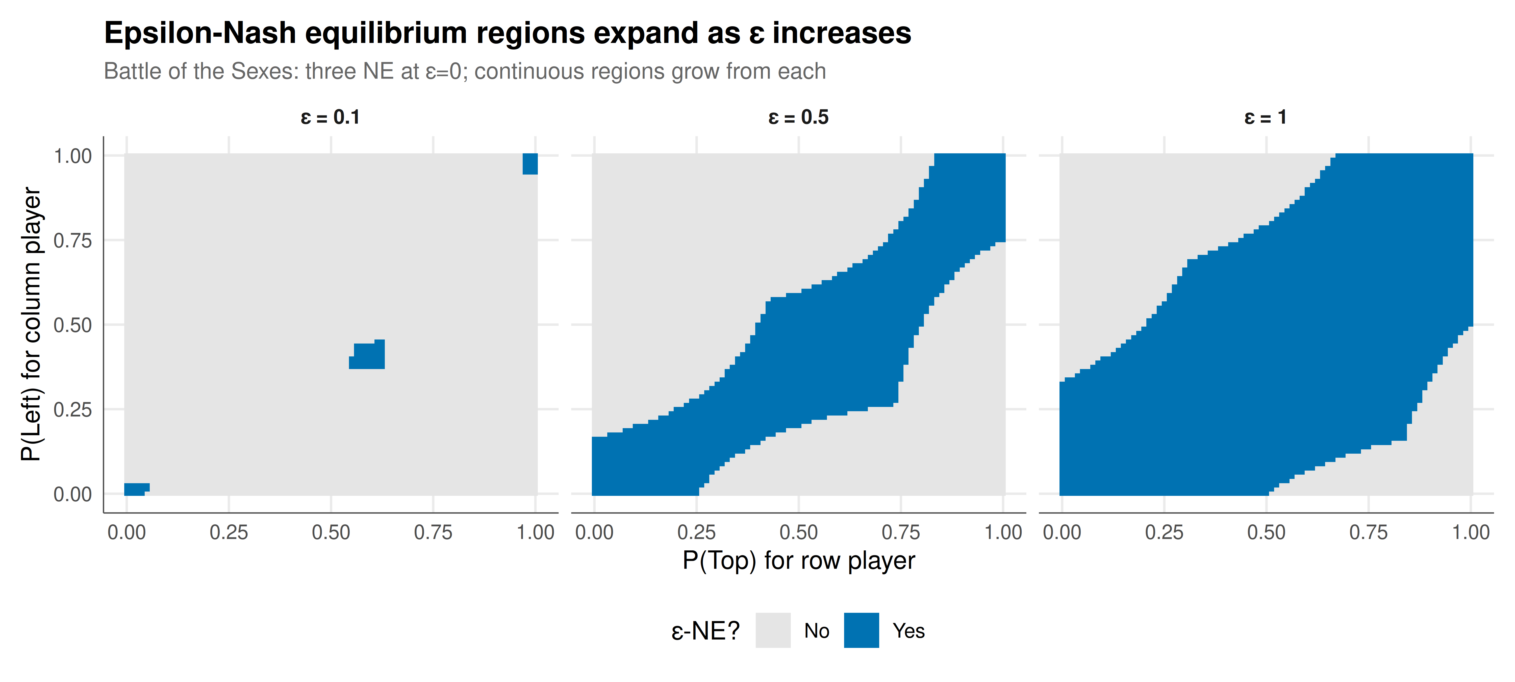
#| fig-cap: "Figure 1. Epsilon-Nash equilibrium regions for the Battle of the Sexes game. Each panel shows the strategy space (p, q) with shading indicating whether each profile is an epsilon-NE. At epsilon=0, only the three Nash equilibria qualify (two pure corners and one mixed). As epsilon increases, the epsilon-NE regions expand from the equilibria, eventually covering the entire strategy space. The mixed NE (p≈0.6, q≈0.4) has a larger basin of approximate equilibrium than the pure NE. Okabe-Ito palette."
#| dev: [png, pdf]
#| fig-width: 10
#| fig-height: 4.5
#| dpi: 300
grid_size <- 81
p_seq <- seq(0, 1, length.out = grid_size)
q_seq <- seq(0, 1, length.out = grid_size)

A_bos <- matrix(c(3, 0, 0, 2), 2, 2)
B_bos <- matrix(c(2, 0, 0, 3), 2, 2)

eps_panels <- c(0.1, 0.5, 1.0)
region_data <- expand.grid(p = p_seq, q = q_seq, epsilon = eps_panels) |>
  as_tibble() |>
  rowwise() |>
  mutate(
    regret = compute_regret(A_bos, B_bos, p, q)["max"],
    is_eps_ne = regret <= epsilon,
    eps_label = paste0("ε = ", epsilon)
  ) |>
  ungroup()

ggplot(region_data, aes(x = p, y = q, fill = is_eps_ne)) +
  geom_tile() +
  facet_wrap(~eps_label) +
  scale_fill_manual(values = c("FALSE" = "grey90", "TRUE" = okabe_ito[5]),
                     name = "ε-NE?", labels = c("No", "Yes")) +
  labs(title = "Epsilon-Nash equilibrium regions expand as ε increases",
       subtitle = "Battle of the Sexes: three NE at ε=0; continuous regions grow from each",
       x = "P(Top) for row player", y = "P(Left) for column player") +
  theme_publication() +
  theme(strip.text = element_text(face = "bold"))
```
## Interactive figure
```{r}
#| label: fig-epsilon-fraction-interactive
# Region size vs epsilon for multiple games
games <- list(
  list(A = A_pd, B = B_pd, name = "Prisoner's Dilemma"),
  list(A = A_bos, B = B_bos, name = "Battle of the Sexes"),
  list(A = A_mp, B = B_mp, name = "Matching Pennies"),
  list(A = matrix(c(2,0,0,1), 2, 2), B = matrix(c(1,0,0,2), 2, 2), name = "Anti-coordination")
)

eps_fine <- seq(0, 2, 0.05)
fraction_data <- lapply(games, function(g) {
  fracs <- sapply(eps_fine, function(e) map_epsilon_ne(g$A, g$B, e, 51))
  tibble(epsilon = eps_fine, fraction = fracs, game = g$name,
         text = paste0("ε = ", round(eps_fine, 2), "\n", g$name,
                       "\nFraction: ", round(fracs * 100, 1), "%"))
}) |> bind_rows()

p_frac <- ggplot(fraction_data, aes(x = epsilon, y = fraction,
                                     color = game, text = text)) +
  geom_line(linewidth = 0.9) +
  scale_color_manual(values = okabe_ito[c(6, 5, 3, 1)], name = NULL) +
  scale_y_continuous(labels = scales::percent_format()) +
  labs(title = "Fraction of strategy space that is ε-Nash equilibrium",
       subtitle = "Games with unique NE expand faster; multiple NE merge at moderate ε",
       x = "Epsilon (ε)", y = "Fraction of (p, q) space") +
  theme_publication()

ggplotly(p_frac, tooltip = "text") |>
  config(displaylogo = FALSE, modeBarButtonsToRemove = c("select2d", "lasso2d"))
```
## Interpretation
Epsilon-equilibrium reveals the "robustness landscape" of strategic interactions. The visualisation of epsilon-NE regions shows that Nash equilibria are not isolated points in strategy space but rather centres of basins of approximate equilibrium. As epsilon increases, these basins expand and eventually merge, revealing which equilibria are most robust to perturbation. In the Battle of the Sexes, the mixed Nash equilibrium has a larger basin than either pure equilibrium at moderate epsilon values — this is surprising because the mixed NE is payoff-dominated and often considered "fragile." But from an approximation standpoint, it is the most central point in strategy space, equidistant from the boundaries where one player's regret becomes large.
The Prisoner's Dilemma illustrates an important asymmetry: mutual cooperation (C,C) is not a Nash equilibrium but becomes an epsilon-NE for relatively small epsilon. With epsilon = 2 (which is large relative to the payoff range), mutual cooperation qualifies. This connects to the experimental observation that subjects often cooperate in one-shot PDs — if the "cost of not best-responding" is small relative to the gains from mutual cooperation, epsilon-equilibrium provides a rationality-compatible explanation for cooperative play without invoking altruism or irrationality.
The comparison across games reveals a structural pattern: games with a unique equilibrium (Matching Pennies, Prisoner's Dilemma) have epsilon-NE regions that grow outward from a single centre, while games with multiple equilibria (Battle of the Sexes) have regions that start separate and merge at a critical epsilon. The merging point indicates the "distance between equilibria" in regret space — a measure of how different the equilibria are from a player's perspective. Games where equilibria merge quickly are strategically simpler than games where they remain separated even at large epsilon.
The computational perspective adds another dimension: since exact Nash equilibrium is PPAD-hard but approximate equilibrium may be easier, epsilon-equilibrium defines a natural "precision-complexity trade-off." Algorithms that find epsilon-NE with epsilon = 0.5 (say, half the payoff range) run in polynomial time, while reducing epsilon to zero requires exponentially more computation in the worst case. This suggests that in large, complex strategic environments (markets with many participants, networks with many nodes), approximate equilibria are not just practically sufficient but computationally necessary — exact equilibria may be theoretically well-defined but practically uncomputable.
## Extensions & related tutorials
- [Nash equilibrium in mixed strategies](../nash-equilibrium-mixed/) — the exact equilibrium that epsilon-NE approximates.
- [Quantal response equilibrium](../../behavioral-gt/quantal-response-equilibrium/) — a smooth approximation model with decision noise.
- [Fictitious play and convergence](../../ml-and-gt/fictitious-play-convergence/) — learning dynamics that converge to epsilon-NE.
- [No-regret learning in games](../../ml-and-gt/no-regret-learning-games/) — algorithms with epsilon-regret guarantees.
- [Lemke-Howson algorithm](../../optimization-numerical-methods/lemke-howson-algorithm/) — exact NE computation (exponential worst case).
## References
::: {#refs}
:::