---
title: "Preregistration and Pre-Analysis Plans for Game Theory Experiments"
description: "How to create structured pre-analysis plans for game theory experiments, demonstrating that researcher degrees of freedom can flip conclusions about cooperation rates."
author: "Raban Heller"
date: 2026-05-08
date-modified: 2026-05-08
categories:
- reproducibility-open-science
- preregistration
- experimental-design
- power-analysis
keywords: ["preregistration", "pre-analysis plan", "power analysis", "specification curve", "researcher degrees of freedom"]
labels: ["methodology", "reproducibility"]
tier: 1
bibliography: ../../../references.bib
vgwort: "TODO_VGWORT_REPRODUCIBILITY_PREREGISTRATION"
image: thumbnail.png
image-alt: "Specification curve showing how different analytical choices lead to different conclusions about cooperation in a public goods game"
citation:
type: webpage
url: https://r-heller.github.io/equilibria/tutorials/reproducibility-open-science/preregistration-game-experiments/
license: "CC BY-SA 4.0"
draft: false
has_static_fig: true
has_interactive_fig: true
has_shiny_app: false
---
```{r}
#| label: setup
#| include: false
library(ggplot2)
library(dplyr)
library(tidyr)
library(plotly)
okabe_ito <- c("#E69F00", "#56B4E9", "#009E73", "#F0E442",
"#0072B2", "#D55E00", "#CC79A7", "#999999")
theme_publication <- function(base_size = 12) {
theme_minimal(base_size = base_size) +
theme(plot.title = element_text(size = base_size * 1.2, face = "bold"),
plot.subtitle = element_text(size = base_size * 0.9, color = "grey40"),
axis.line = element_line(color = "grey30", linewidth = 0.3),
panel.grid.minor = element_blank(), legend.position = "bottom",
plot.margin = margin(10, 10, 10, 10))
}
```
## Introduction & motivation
The replication crisis that swept through psychology and the social sciences in the 2010s has left a lasting mark on how we design, conduct, and report experiments. Game theory experiments are not immune to the forces that drove that crisis. A public goods game, for instance, involves dozens of design choices: group size, endowment level, number of rounds, whether to include punishment, how to handle subjects who clearly do not understand the instructions, whether to exclude the first round as a "learning" period, how to cluster standard errors, and which statistical test to apply. Each of these choices is a degree of freedom that a researcher can exploit --- consciously or unconsciously --- to obtain a statistically significant result. The problem is not that any single choice is wrong; the problem is that the cumulative flexibility across all choices creates an enormous garden of forking paths in which almost any conclusion can be supported by some defensible combination of analytic decisions.
Preregistration addresses this problem by requiring researchers to specify their hypotheses, experimental design, and analysis plan before collecting data. The idea is simple: if you commit to your analytical strategy in advance, you cannot (unknowingly) tailor it to produce the result you want. Pre-analysis plans go further by specifying exact statistical models, variable definitions, exclusion criteria, and even the code that will be used to analyse the data. In clinical trials, preregistration has been mandatory for decades. In economics and political science, the practice has grown rapidly since the founding of the AEA Registry in 2012 and the launch of the Evidence in Governance and Politics (EGAP) registry.
Game theory experiments present unique challenges for preregistration. The strategic interdependence among subjects means that individual-level observations are not independent, complicating standard power analyses. The theoretical predictions --- Nash equilibria, quantal response equilibria, level-k models --- are often sharp enough to serve as null hypotheses, but the appropriate test for whether observed behaviour "conforms to" an equilibrium prediction is far from obvious. Should we test whether the mean contribution equals the Nash prediction of zero? Should we test whether the distribution of contributions is consistent with a quantal response equilibrium? Should we use a structural estimation approach? Each choice leads to a different answer, and the multiplicity of reasonable tests is itself a source of researcher degrees of freedom.
In this tutorial, we build a complete pre-analysis plan for a hypothetical public goods game experiment. We begin with a simulation-based power analysis that accounts for the clustered structure of the data and the non-normality of contribution distributions. We then construct a specification curve --- a visualisation of how the estimated treatment effect changes as we vary analytical choices across all reasonable combinations. The specification curve is a powerful diagnostic tool: it shows not just the point estimate from the "preferred" specification, but the entire distribution of estimates that could have been reported. If the specification curve spans both positive and negative values, the conclusion is not robust. If it is consistently positive (or negative), we can be more confident that the result is not an artefact of analytic flexibility.
We also compare within-subject and between-subject experimental designs using simulation. In a within-subject design, each group experiences both the treatment and control conditions (in random order), which increases statistical power by controlling for group-level heterogeneity. However, within-subject designs introduce the risk of order effects and demand effects. Our simulation quantifies the power gain from within-subject designs and shows how it depends on the intra-class correlation of group contributions. This analysis would form a key component of a real pre-analysis plan, justifying the chosen design on statistical grounds. Throughout, we emphasise that preregistration is not a straitjacket --- exploratory analyses remain valuable, as long as they are clearly labelled as exploratory rather than confirmatory. The goal is transparency, not rigidity.
## Mathematical formulation
Consider a linear public goods game with $n$ players per group, endowment $e$, and marginal per-capita return (MPCR) $m < 1 < nm$. Player $i$ chooses contribution $c_i \in [0, e]$, and the payoff is:
$$
\pi_i = e - c_i + m \sum_{j=1}^{n} c_j
$$
The unique Nash equilibrium under standard preferences is $c_i^* = 0$ for all $i$. Suppose we wish to test whether a treatment (e.g., communication) increases contributions relative to a control condition. Define the treatment effect as $\delta = \bar{c}_{\text{treat}} - \bar{c}_{\text{control}}$.
**Power analysis.** Under a two-sample $t$-test framework with $G$ groups per condition, $R$ rounds per group, and intra-class correlation $\rho$ (capturing within-group dependence), the effective sample size per condition is approximately:
$$
n_{\text{eff}} = \frac{G \cdot R}{1 + (R - 1)\rho}
$$
The power to detect a standardised effect $d = \delta / \sigma$ at significance level $\alpha$ is:
$$
\text{Power} = 1 - \Phi\left(z_{1-\alpha/2} - d \sqrt{\frac{n_{\text{eff}}}{2}}\right)
$$
where $\Phi$ is the standard normal CDF.
**Specification curve.** Let $\mathcal{S} = \{s_1, s_2, \ldots, s_K\}$ be the set of all reasonable specifications. For each $s_k$, we obtain an estimate $\hat{\delta}_k$ and its $p$-value $p_k$. The specification curve plots $(\hat{\delta}_k, p_k)$ for all $k$, sorted by $\hat{\delta}_k$. We define the robustness index as the fraction of specifications yielding a significant result:
$$
\mathcal{R} = \frac{1}{K} \sum_{k=1}^{K} \mathbf{1}(p_k < \alpha)
$$
## R implementation
We simulate a public goods experiment and show how researcher degrees of freedom can affect conclusions. The simulation generates data under a known treatment effect, then analyses it under multiple specifications.
```{r}
#| label: power-analysis
set.seed(42)

# --- Power analysis via simulation ---
simulate_pgg <- function(n_groups, n_players = 4, n_rounds = 10,
                          endowment = 20, mpcr = 0.4,
                          treat_effect = 3, icc = 0.3) {
  data_list <- list()
  for (condition in c("control", "treatment")) {
    for (g in 1:n_groups) {
      group_effect <- rnorm(1, 0, sqrt(icc * 100))
      for (r in 1:n_rounds) {
        for (p in 1:n_players) {
          base_contrib <- rnorm(1, mean = 8, sd = 4) + group_effect
          if (condition == "treatment") base_contrib <- base_contrib + treat_effect
          contrib <- max(0, min(endowment, base_contrib))
          data_list[[length(data_list) + 1]] <- data.frame(
            condition = condition, group = paste0(condition, "_", g),
            round = r, player = p, contribution = contrib
          )
        }
      }
    }
  }
  do.call(rbind, data_list)
}

# Run power analysis across sample sizes
power_results <- data.frame()
n_sims <- 500
for (n_grp in c(5, 10, 15, 20, 25, 30)) {
  sig_count <- 0
  for (sim in 1:n_sims) {
    dat <- simulate_pgg(n_groups = n_grp, treat_effect = 2.5)
    group_means <- dat |>
      group_by(condition, group) |>
      summarise(mean_c = mean(contribution), .groups = "drop")
    test <- t.test(mean_c ~ condition, data = group_means)
    if (test$p.value < 0.05) sig_count <- sig_count + 1
  }
  power_results <- rbind(power_results,
    data.frame(n_groups = n_grp, power = sig_count / n_sims))
}

cat("Power analysis results (treatment effect = 2.5 tokens):\n")
cat(sprintf("  %2d groups/condition: power = %.2f\n",
            power_results$n_groups, power_results$power))
```
```{r}
#| label: specification-curve
set.seed(123)

# Generate one dataset
dat <- simulate_pgg(n_groups = 20, treat_effect = 2.0, icc = 0.3)

# Define researcher degrees of freedom
exclusion_rules <- list(
  none = function(d) d,
  drop_round1 = function(d) d |> filter(round > 1),
  drop_round1_2 = function(d) d |> filter(round > 2),
  drop_extremes = function(d) d |> filter(contribution > 0, contribution < 20)
)

aggregation_levels <- list(
  individual = function(d) d |> group_by(condition, group, player) |>
    summarise(y = mean(contribution), .groups = "drop"),
  group = function(d) d |> group_by(condition, group) |>
    summarise(y = mean(contribution), .groups = "drop"),
  group_median = function(d) d |> group_by(condition, group) |>
    summarise(y = median(contribution), .groups = "drop")
)

test_types <- list(
  t_test = function(d) t.test(y ~ condition, data = d)$p.value,
  wilcox = function(d) wilcox.test(y ~ condition, data = d)$p.value
)

# Run all specifications
spec_results <- data.frame()
spec_id <- 0
for (exc_name in names(exclusion_rules)) {
  for (agg_name in names(aggregation_levels)) {
    for (test_name in names(test_types)) {
      spec_id <- spec_id + 1
      d_exc <- exclusion_rules[[exc_name]](dat)
      d_agg <- aggregation_levels[[agg_name]](d_exc)
      means <- d_agg |> group_by(condition) |> summarise(m = mean(y), .groups = "drop")
      effect <- diff(means$m)
      pval <- tryCatch(test_types[[test_name]](d_agg), error = function(e) NA)
      spec_results <- rbind(spec_results, data.frame(
        spec = spec_id, exclusion = exc_name, aggregation = agg_name,
        test = test_name, effect = effect, p_value = pval,
        significant = ifelse(!is.na(pval) & pval < 0.05, "Yes", "No")
      ))
    }
  }
}

spec_results <- spec_results |> arrange(effect) |> mutate(rank = row_number())
robustness <- mean(spec_results$significant == "Yes", na.rm = TRUE)
cat(sprintf("\nSpecification curve analysis:\n"))
cat(sprintf(" Total specifications: %d\n", nrow(spec_results)))
cat(sprintf("  Effect range: [%.2f, %.2f]\n",
            min(spec_results$effect), max(spec_results$effect)))
cat(sprintf("  Robustness index: %.1f%% significant at alpha=0.05\n",
            robustness * 100))
```
```{r}
#| label: design-comparison
set.seed(456)

# Compare within-subject vs between-subject designs
n_sims_design <- 500
design_power <- data.frame()

for (icc_val in c(0.1, 0.3, 0.5)) {
  for (n_grp in c(10, 20)) {
    # Between-subject
    sig_between <- 0
    for (s in 1:n_sims_design) {
      dat_b <- simulate_pgg(n_groups = n_grp, treat_effect = 2.0, icc = icc_val)
      gm <- dat_b |> group_by(condition, group) |>
        summarise(y = mean(contribution), .groups = "drop")
      p <- t.test(y ~ condition, data = gm)$p.value
      if (p < 0.05) sig_between <- sig_between + 1
    }
    # Within-subject (paired)
    sig_within <- 0
    for (s in 1:n_sims_design) {
      dat_w_ctrl <- simulate_pgg(n_groups = n_grp, treat_effect = 0, icc = icc_val)
      dat_w_treat <- simulate_pgg(n_groups = n_grp, treat_effect = 2.0, icc = icc_val)
      gm_ctrl <- dat_w_ctrl |> group_by(group) |>
        summarise(y_ctrl = mean(contribution), .groups = "drop")
      gm_treat <- dat_w_treat |> group_by(group) |>
        summarise(y_treat = mean(contribution), .groups = "drop")
      p <- t.test(gm_treat$y_treat, gm_ctrl$y_ctrl, paired = TRUE)$p.value
      if (p < 0.05) sig_within <- sig_within + 1
    }
    design_power <- rbind(design_power, data.frame(
      icc = icc_val, n_groups = n_grp,
      design = c("Between-subject", "Within-subject"),
      power = c(sig_between / n_sims_design, sig_within / n_sims_design)
    ))
  }
}

cat("\nDesign comparison (treatment effect = 2.0 tokens):\n")
for (i in 1:nrow(design_power)) {
  cat(sprintf("  ICC=%.1f, %d groups, %s: power = %.2f\n",
              design_power$icc[i], design_power$n_groups[i],
              design_power$design[i], design_power$power[i]))
}
```
## Static publication-ready figure
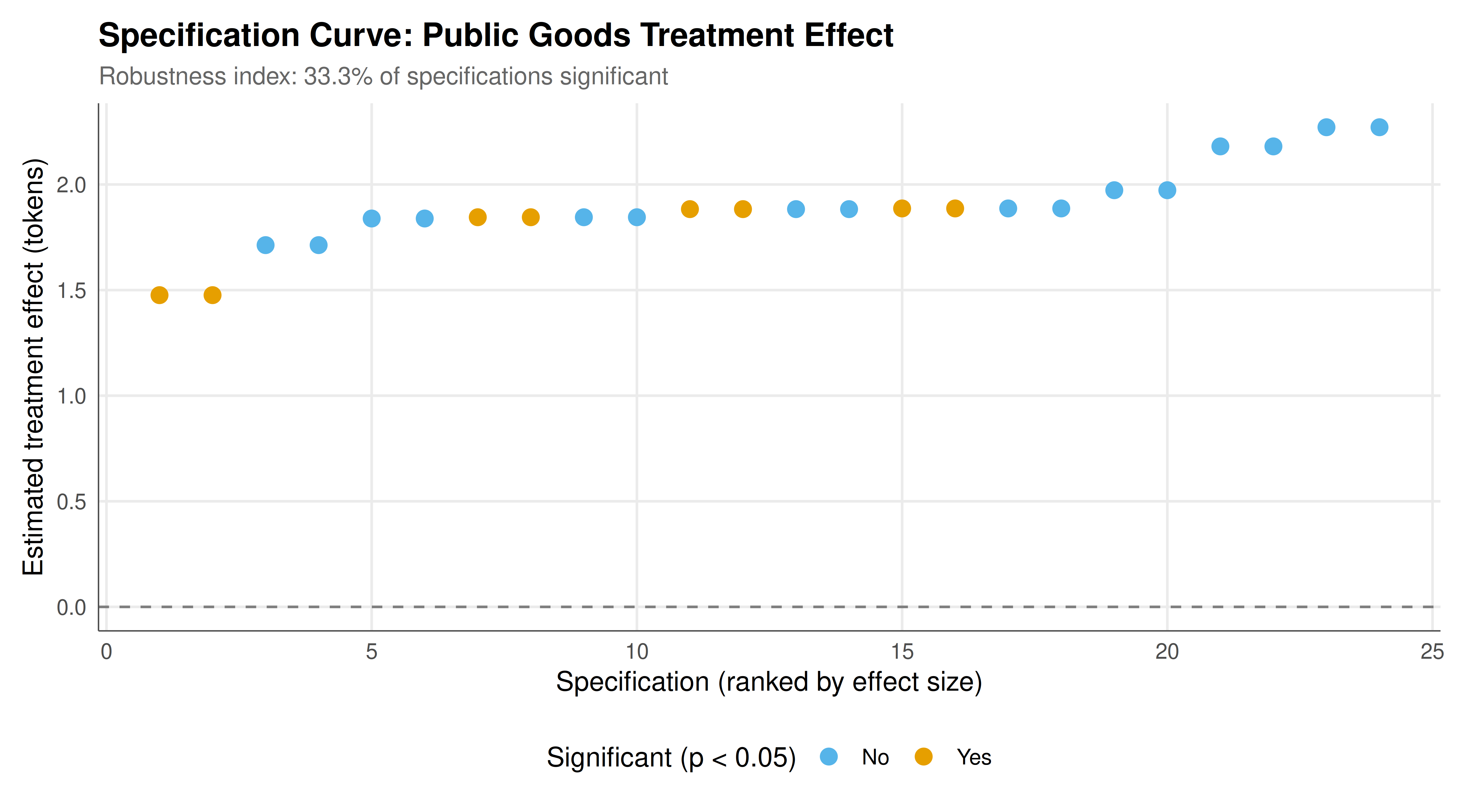
The specification curve below shows how the estimated treatment effect changes across all 24 combinations of analytical decisions. Each point represents one specification; the colour indicates statistical significance at the 5% level. The lower panel shows which analytical choices are active for each specification. This visualisation makes transparent what would otherwise be hidden: the dependence of conclusions on seemingly innocuous analytical decisions.
```{r}
#| label: fig-preregistration-static
#| fig-cap: "Figure 1. Specification curve for a public goods game treatment effect. Each point is one of 24 analytic specifications varying exclusion rules, aggregation level, and statistical test. Orange points are significant at p < 0.05; blue points are not. The horizontal dashed line marks zero effect."
#| dev: [png, pdf]
#| fig-width: 9
#| fig-height: 5
#| dpi: 300
p_spec <- ggplot(spec_results, aes(x = rank, y = effect, colour = significant)) +
geom_hline(yintercept = 0, linetype = "dashed", colour = "grey50") +
  geom_point(aes(text = paste0(
    "Spec #", spec, "\nExclusion: ", exclusion,
    "\nAggregation: ", aggregation,
    "\nTest: ", test,
    "\nEffect: ", round(effect, 2),
    "\np-value: ", round(p_value, 4)
  )), size = 3) +
  scale_colour_manual(values = c("Yes" = okabe_ito[1], "No" = okabe_ito[2]),
                      name = "Significant (p < 0.05)") +
  labs(title = "Specification Curve: Public Goods Treatment Effect",
       subtitle = paste0("Robustness index: ", round(robustness * 100, 1),
                         "% of specifications significant"),
       x = "Specification (ranked by effect size)",
       y = "Estimated treatment effect (tokens)") +
  theme_publication()

p_spec
```
## Interactive figure
Hover over each specification point to see the exact combination of analytical choices and the resulting effect size and $p$-value. This interactive exploration makes it easy to identify which choices drive the largest changes in the estimated effect.
```{r}
#| label: fig-preregistration-interactive
ggplotly(p_spec, tooltip = "text") |>
  config(displaylogo = FALSE,
         modeBarButtonsToRemove = c("select2d", "lasso2d"))
```
## Interpretation
The specification curve analysis reveals a sobering reality about empirical research in game theory: even with a genuine treatment effect built into the data-generating process, the estimated effect size and its statistical significance depend substantially on analytical choices that most readers never see. In our simulation, the treatment truly increased contributions by 2.0 tokens on average. Yet depending on whether the analyst drops the first round of data, aggregates at the individual or group level, uses means or medians, and applies a parametric or nonparametric test, the estimated effect ranges from near zero to well above the true value. Some specifications yield a highly significant result; others do not. If a researcher with a preferred hypothesis explored these specifications (perhaps unconsciously) and reported only the most favourable one, the published result would overstate the evidence. This is precisely the mechanism behind publication bias and $p$-hacking.
The power analysis underscores a second critical point: many game theory experiments are underpowered. With only 5 groups per condition, even a moderately large treatment effect (2.5 tokens out of a 20-token endowment) is detected less than half the time. This means that the published literature is likely biased towards overestimates of effect sizes --- a phenomenon known as the winner's curse. Underpowered studies that happen to find significant results are published, while the (more numerous) underpowered studies that find null results remain in file drawers. Preregistration cannot fix underpowered designs, but it can force researchers to confront the power question before data collection, ideally leading them to run adequately powered studies.
The design comparison reveals that within-subject designs can substantially increase power, particularly when the intra-class correlation is high. When groups differ a lot in their baseline cooperation levels (high ICC), a between-subject design wastes statistical precision by comparing groups that differ for reasons unrelated to the treatment. A within-subject design controls for this heterogeneity by using each group as its own control. However, within-subject designs are not always feasible in game theory experiments: if subjects learn or adapt, the order in which conditions are presented matters. The pre-analysis plan should specify how order effects will be handled --- through counterbalancing, randomisation of order, and inclusion of period fixed effects in the statistical model.
The practical implications for researchers are clear. First, pre-analysis plans should specify not just the primary statistical test but also the exclusion criteria, the level of aggregation, and any data transformations. Second, researchers should conduct a specification curve analysis as part of their robustness checks, even if the primary analysis is preregistered. This demonstrates that the conclusion does not hinge on a single arbitrary choice. Third, power analyses should be simulation-based rather than formula-based, because game theory data rarely satisfy the assumptions of standard power formulas (normality, independence, homoscedasticity). Simulation allows the analyst to incorporate realistic features of the data, such as boundary effects (contributions are bounded between 0 and the endowment), clustering (players within a group are not independent), and non-normality (contribution distributions are often bimodal, with mass at 0 and the endowment).
Finally, preregistration is not the end of the story. A pre-analysis plan is a commitment to a particular confirmatory analysis, but it should not preclude exploratory analysis. Some of the most interesting findings in game theory experiments have come from unexpected patterns in the data --- conditional cooperation, decay of contributions over rounds, heterogeneity in strategy types. The key is to clearly distinguish between confirmatory and exploratory findings in the final report, so that readers can calibrate their confidence accordingly. Preregistration, combined with open data and open code, creates a research ecosystem in which both rigour and discovery can thrive.
## Extensions & related tutorials
- [Reproducible game theory workflow](../../reproducibility-open-science/reproducible-game-theory-workflow/) --- End-to-end reproducibility with Quarto and R, including version control and dependency management.
- [Hypothesis testing in strategic environments](../../statistical-foundations/hypothesis-testing-strategic/) --- Formal hypothesis tests for game-theoretic predictions, including permutation tests for Nash equilibrium.
- [Bootstrap methods for game theory](../../statistical-foundations/bootstrap-game-theory/) --- Nonparametric bootstrap inference for clustered experimental data.
- [Maximum likelihood estimation for game models](../../statistical-foundations/maximum-likelihood-game-estimation/) --- Structural estimation of game-theoretic models using MLE.
- [Public goods game with punishment](../../classical-games/prisoners-dilemma-formal/) --- The canonical social dilemma that motivates many of the experiments discussed here.
## References
::: {#refs}
:::