---
title: "Hypothesis Testing in Strategic Environments"
description: "Frame statistical hypothesis testing as a game between researcher and Nature, implement permutation tests for Nash equilibrium deviations, and demonstrate multiple testing corrections across games."
author: "Raban Heller"
date: 2026-05-08
date-modified: 2026-05-08
categories:
- statistical-foundations
- hypothesis-testing
- nash-equilibrium
- permutation-test
keywords: ["hypothesis testing", "Neyman-Pearson", "minimax", "permutation test", "multiple testing", "Nash equilibrium"]
labels: ["statistics", "methodology"]
tier: 1
bibliography: ../../../references.bib
vgwort: "TODO_VGWORT_STATISTICS_HYPOTHESIS"
image: thumbnail.png
image-alt: "Power curves for detecting deviations from Nash equilibrium predictions across different sample sizes"
citation:
type: webpage
url: https://r-heller.github.io/equilibria/tutorials/statistical-foundations/hypothesis-testing-strategic/
license: "CC BY-SA 4.0"
draft: false
has_static_fig: true
has_interactive_fig: true
has_shiny_app: false
---
```{r}
#| label: setup
#| include: false
library(ggplot2)
library(dplyr)
library(tidyr)
library(plotly)
okabe_ito <- c("#E69F00", "#56B4E9", "#009E73", "#F0E442",
"#0072B2", "#D55E00", "#CC79A7", "#999999")
theme_publication <- function(base_size = 12) {
theme_minimal(base_size = base_size) +
theme(plot.title = element_text(size = base_size * 1.2, face = "bold"),
plot.subtitle = element_text(size = base_size * 0.9, color = "grey40"),
axis.line = element_line(color = "grey30", linewidth = 0.3),
panel.grid.minor = element_blank(), legend.position = "bottom",
plot.margin = margin(10, 10, 10, 10))
}
```
## Introduction & motivation
Statistical hypothesis testing and game theory share a deep intellectual lineage. Abraham Wald, in his foundational work on statistical decision theory in the 1940s and 1950s, explicitly framed hypothesis testing as a two-person zero-sum game between a statistician (the decision-maker) and Nature (the adversary who chooses the true state of the world). In this framework, the statistician chooses a decision rule --- a mapping from data to actions --- and Nature chooses the true parameter value. The statistician's loss depends on both choices: rejecting a true null hypothesis (Type I error) or failing to reject a false one (Type II error). The minimax approach seeks the decision rule that minimises the maximum possible loss, treating Nature as a hostile opponent. This game-theoretic perspective is not merely a mathematical curiosity; it provides the conceptual foundation for the Neyman-Pearson framework that dominates modern statistical practice.
In experimental game theory, hypothesis testing takes on an additional layer of complexity. The researcher's hypotheses are themselves derived from game-theoretic models. A typical null hypothesis might be: "subjects play according to the mixed-strategy Nash equilibrium." Testing this hypothesis requires specifying what "according to" means. Do we test whether the average mixing probability equals the equilibrium prediction? Do we test whether each individual's choice frequencies are consistent with the equilibrium? Do we test the joint distribution of choices across all subjects? Each formulation leads to a different test with different statistical properties, and the choice among them is a substantive modelling decision rather than a purely statistical one.
Permutation tests offer a particularly attractive approach for testing game-theoretic predictions. Unlike parametric tests, which assume a specific distributional form for the data, permutation tests are exact in finite samples under the null hypothesis of exchangeability. The basic idea is simple: if the null hypothesis is true (e.g., if two groups of subjects are playing the same game and should behave identically), then the assignment of observations to groups is arbitrary, and any permutation of the group labels is equally likely. By computing the test statistic for all (or a large random sample of) permutations, we obtain the null distribution of the test statistic without assuming normality, homoscedasticity, or any other parametric condition. This is particularly valuable in game theory experiments, where the data are often highly non-normal --- subjects in a matching pennies experiment, for example, choose either Heads or Tails, producing binary data that is far from Gaussian.
A further challenge arises when the researcher tests hypotheses across multiple games simultaneously. In a typical experimental paper, subjects might play several different $2 \times 2$ games, and the researcher tests whether behaviour conforms to the Nash equilibrium prediction in each game. If the researcher uses a significance level of $\alpha = 0.05$ for each test, the probability of at least one false rejection grows rapidly with the number of tests --- the multiple comparisons problem. Without correction, a researcher testing 20 games would expect to find one "significant deviation from Nash equilibrium" even if subjects play exactly according to theory in every game. The Bonferroni correction, the Holm-Bonferroni procedure, and the Benjamini-Hochberg false discovery rate (FDR) procedure address this problem by adjusting the significance threshold, but at the cost of reducing power. The choice of correction method is yet another researcher degree of freedom that must be specified in advance (ideally in a pre-analysis plan) to avoid $p$-hacking.
In this tutorial, we bring these ideas together. We implement the Neyman-Pearson framework as a minimax problem, compute power curves for detecting deviations from Nash equilibrium, build a permutation test for mixed-strategy NE predictions in a matching pennies game, and demonstrate three multiple testing corrections across a battery of games. The goal is to equip the reader with practical tools for rigorous hypothesis testing in game-theoretic contexts, while illuminating the game-theoretic structure of hypothesis testing itself.
## Mathematical formulation
**Hypothesis testing as a game.** The researcher chooses a test $\phi: \mathcal{X} \to \{0, 1\}$ (reject or not). Nature chooses $\theta \in \Theta$. The loss function is:
$$
L(\phi, \theta) = \begin{cases} \alpha(\phi) & \text{if } \theta \in \Theta_0 \text{ (Type I error)} \\ \beta(\phi, \theta) & \text{if } \theta \in \Theta_1 \text{ (Type II error)} \end{cases}
$$
where $\alpha(\phi) = \mathbb{E}_{\theta_0}[\phi(X)]$ is the size and $\beta(\phi, \theta) = 1 - \mathbb{E}_\theta[\phi(X)]$ is one minus the power. The **minimax test** solves:
$$
\min_{\phi: \alpha(\phi) \leq \alpha_0} \max_{\theta \in \Theta_1} \beta(\phi, \theta)
$$
**Permutation test for NE.** Consider a matching pennies game with NE prediction $p^* = 0.5$ (probability of playing Heads). We observe $n$ choices $X_1, \ldots, X_n \in \{H, T\}$. The test statistic is:
$$
T = \left| \hat{p} - p^* \right| = \left| \frac{1}{n}\sum_{i=1}^n \mathbf{1}(X_i = H) - 0.5 \right|
$$
Under $H_0: p = p^*$, the exact null distribution of $T$ is derived from the binomial distribution $\text{Bin}(n, 0.5)$.
**Multiple testing corrections.** Given $m$ tests with $p$-values $p_1, \ldots, p_m$:
- **Bonferroni:** Reject $H_{0,j}$ if $p_j < \alpha / m$.
- **Holm-Bonferroni:** Order $p$-values: $p_{(1)} \leq \cdots \leq p_{(m)}$. Reject $H_{0,(j)}$ if $p_{(j)} < \alpha / (m - j + 1)$ for all preceding hypotheses.
- **Benjamini-Hochberg (FDR):** Reject $H_{0,(j)}$ if $p_{(j)} \leq j \cdot \alpha / m$ for the largest such $j$ and all $p$-values below it.
## R implementation
We implement the minimax power analysis, a permutation test for Nash equilibrium, and multiple testing corrections across a battery of games.
```{r}
#| label: power-analysis-minimax
set.seed(314)

# --- Power curves for detecting deviations from NE ---
# Matching pennies: NE predicts p = 0.5
# H0: p = 0.5 vs H1: p != 0.5
# Test: exact binomial test

compute_power <- function(n, p_true, p_null = 0.5, alpha = 0.05) {
  # Power via simulation
  n_sims <- 5000
  rejections <- 0
  for (s in 1:n_sims) {
    x <- rbinom(1, n, p_true)
    pval <- binom.test(x, n, p = p_null)$p.value
    if (pval < alpha) rejections <- rejections + 1
  }
  rejections / n_sims
}

# Grid of sample sizes and true probabilities
sample_sizes <- c(20, 50, 100, 200)
p_true_values <- seq(0.3, 0.7, by = 0.02)

power_data <- expand.grid(n = sample_sizes, p_true = p_true_values) |>
  mutate(power = mapply(compute_power, n, p_true))

cat("Power at selected points (alpha = 0.05):\n")
for (nn in sample_sizes) {
  pw <- power_data |> filter(n == nn, p_true == 0.6)
  cat(sprintf("  n = %3d, p_true = 0.60: power = %.3f\n", nn, pw$power))
}
```
```{r}
#| label: permutation-test
set.seed(271)

# --- Permutation test: does observed play differ from mixed NE? ---
# Simulate data from a matching pennies experiment
n_subjects <- 40
n_rounds <- 50

# True behavior: subjects play H with probability 0.55 (slight deviation from NE)
simulated_data <- data.frame(
  subject = rep(1:n_subjects, each = n_rounds),
  round = rep(1:n_rounds, n_subjects),
  choice = rbinom(n_subjects * n_rounds, 1, 0.55)  # 1 = Heads
)

# Observed aggregate proportion
obs_p <- mean(simulated_data$choice)
obs_stat <- abs(obs_p - 0.5)

# Permutation test: under H0, each choice is equally likely H or T
# Resample from Bernoulli(0.5)
n_perms <- 10000
perm_stats <- numeric(n_perms)
for (i in 1:n_perms) {
  perm_choices <- rbinom(n_subjects * n_rounds, 1, 0.5)
  perm_p <- mean(perm_choices)
  perm_stats[i] <- abs(perm_p - 0.5)
}

perm_pvalue <- mean(perm_stats >= obs_stat)

cat(sprintf("\nPermutation test for Nash equilibrium (p* = 0.5):\n"))
cat(sprintf(" Observed proportion Heads: %.4f\n", obs_p))
cat(sprintf(" Test statistic |p_hat - 0.5|: %.4f\n", obs_stat))
cat(sprintf(" Permutation p-value: %.4f\n", perm_pvalue))
cat(sprintf("  Conclusion: %s at alpha = 0.05\n",
    ifelse(perm_pvalue < 0.05, "Reject H0 (behaviour differs from NE)",
           "Fail to reject H0")))
```
```{r}
#| label: multiple-testing
set.seed(159)

# --- Multiple testing across a battery of games ---
# Simulate 12 games, each with a NE prediction for p(Heads)
games <- data.frame(
  game = paste0("Game_", sprintf("%02d", 1:12)),
  p_ne = c(0.5, 0.5, 0.75, 0.25, 0.5, 0.67, 0.33, 0.5, 0.5, 0.6, 0.4, 0.5),
  p_true = c(0.52, 0.55, 0.73, 0.30, 0.48, 0.70, 0.35, 0.50, 0.53, 0.58, 0.42, 0.51),
  n_obs = rep(200, 12)
)

# Generate p-values
games <- games |>
  rowwise() |>
  mutate(
    x = rbinom(1, n_obs, p_true),
    p_value = binom.test(x, n_obs, p = p_ne)$p.value
  ) |>
  ungroup()

# Apply corrections
games <- games |>
  mutate(
    p_bonferroni = p.adjust(p_value, method = "bonferroni"),
    p_holm = p.adjust(p_value, method = "holm"),
    p_bh = p.adjust(p_value, method = "BH"),
    sig_raw = p_value < 0.05,
    sig_bonferroni = p_bonferroni < 0.05,
    sig_holm = p_holm < 0.05,
    sig_bh = p_bh < 0.05
  )

cat("\nMultiple testing corrections across 12 games:\n")
cat(sprintf(" Significant (raw): %d / %d\n", sum(games$sig_raw), nrow(games)))
cat(sprintf(" Significant (Bonferroni): %d / %d\n", sum(games$sig_bonferroni), nrow(games)))
cat(sprintf(" Significant (Holm): %d / %d\n", sum(games$sig_holm), nrow(games)))
cat(sprintf(" Significant (BH FDR): %d / %d\n", sum(games$sig_bh), nrow(games)))
cat("\nDetailed results:\n")
for (i in 1:nrow(games)) {
  cat(sprintf("  %s: p_NE=%.2f, p_obs=%.3f, raw_p=%.4f, BH=%.4f %s\n",
              games$game[i], games$p_ne[i], games$x[i] / games$n_obs[i],
              games$p_value[i], games$p_bh[i],
              ifelse(games$sig_bh[i], "*", "")))
}
```
## Static publication-ready figure
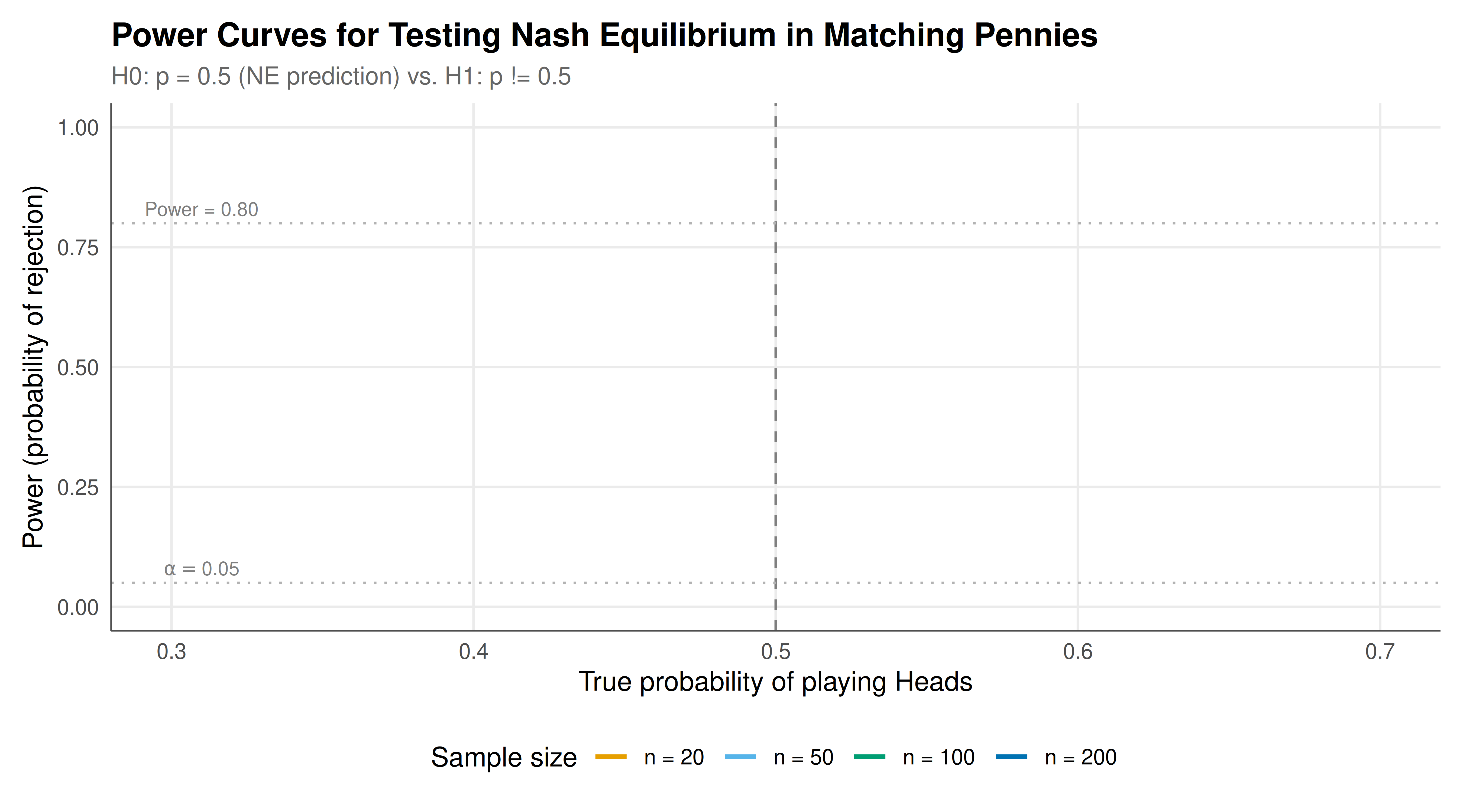
The power curve plot below shows how the probability of detecting a deviation from Nash equilibrium depends on the true mixing probability and the sample size. At the Nash equilibrium ($p = 0.5$), the rejection rate equals the significance level (5%), confirming correct size control. As the true probability moves away from 0.5, power increases, with larger samples detecting smaller deviations.
```{r}
#| label: fig-hypothesis-static
#| fig-cap: "Figure 1. Power curves for detecting deviations from the mixed-strategy Nash equilibrium (p = 0.5) in a matching pennies game. Each curve corresponds to a different sample size. Vertical dashed line marks the NE prediction. Power equals the significance level (0.05) at the null, and increases as the true probability deviates from 0.5."
#| dev: [png, pdf]
#| fig-width: 9
#| fig-height: 5
#| dpi: 300
power_data <- power_data |>
  mutate(n_label = factor(paste0("n = ", n), levels = paste0("n = ", sample_sizes)))

p_power <- ggplot(power_data, aes(x = p_true, y = power, colour = n_label,
    text = paste0("n = ", n, "\np_true = ", p_true,
                  "\nPower = ", round(power, 3)))) +
  geom_line(linewidth = 0.9) +
  geom_vline(xintercept = 0.5, linetype = "dashed", colour = "grey50") +
  geom_hline(yintercept = 0.05, linetype = "dotted", colour = "grey70") +
  geom_hline(yintercept = 0.80, linetype = "dotted", colour = "grey70") +
  scale_colour_manual(values = okabe_ito[c(1, 2, 3, 5)], name = "Sample size") +
  annotate("text", x = 0.31, y = 0.08, label = "alpha == 0.05",
           parse = TRUE, size = 3, colour = "grey50") +
  annotate("text", x = 0.31, y = 0.83, label = "Power = 0.80",
           size = 3, colour = "grey50") +
  labs(title = "Power Curves for Testing Nash Equilibrium in Matching Pennies",
       subtitle = "H0: p = 0.5 (NE prediction) vs. H1: p != 0.5",
       x = "True probability of playing Heads",
       y = "Power (probability of rejection)") +
  coord_cartesian(ylim = c(0, 1)) +
  theme_publication()

p_power
```
## Interactive figure
Hover over the power curves to see exact power values for each combination of sample size and true probability. This makes it easy to determine the sample size needed to achieve 80% power for a given deviation from Nash equilibrium.
```{r}
#| label: fig-hypothesis-interactive
ggplotly(p_power, tooltip = "text") |>
  config(displaylogo = FALSE,
         modeBarButtonsToRemove = c("select2d", "lasso2d"))
```
## Interpretation
The results of this tutorial illuminate the deep connections between statistical hypothesis testing and game theory, both conceptually and practically. The framing of hypothesis testing as a game between researcher and Nature is more than an elegant metaphor; it provides a rigorous decision-theoretic foundation for choosing among statistical procedures. The minimax criterion, which selects the test that performs best in the worst case, is conservative but robust. It is appropriate when the researcher has no prior information about which alternative hypothesis is most plausible --- analogous to playing a maxmin strategy in a zero-sum game. When prior information is available (e.g., from previous experiments or theoretical predictions), Bayesian approaches that assign prior probabilities to different parameter values may be more efficient. The choice between minimax and Bayesian approaches is itself a decision that should be justified in the pre-analysis plan.
The power analysis reveals a key practical challenge for experimental game theory: detecting small deviations from Nash equilibrium requires large samples. If the true mixing probability in a matching pennies game is 0.55 (a 5-percentage-point deviation from the NE prediction of 0.50), a sample of 200 observations achieves only moderate power. To reliably detect such a deviation with 80% power, we need several hundred observations. This is problematic because many game theory experiments use relatively small samples --- 20 to 50 subjects playing 10 to 20 rounds. With such sample sizes, only large deviations from the NE prediction can be detected, and failure to reject the null hypothesis is ambiguous: it could mean that subjects play according to Nash, or it could mean that the test lacks the power to detect departures. Reporting confidence intervals alongside $p$-values is essential for resolving this ambiguity: a wide confidence interval that includes both the NE prediction and large deviations indicates insufficient power, while a narrow confidence interval centred on the NE prediction provides genuine evidence of equilibrium play.
The permutation test demonstrates a non-parametric approach that is particularly well-suited to game theory data. Because the null hypothesis of Nash equilibrium play makes a sharp prediction about the data-generating process (each choice is an independent Bernoulli draw with probability $p^*$), we can construct the null distribution of any test statistic by simulation. The permutation test is exact in finite samples, requires no distributional assumptions beyond exchangeability, and can be applied to any test statistic --- not just the sample mean. For example, we could test whether the serial correlation of choices (a pattern inconsistent with independent mixing) differs from zero, or whether the distribution of choice frequencies across subjects is consistent with a common mixing probability. The flexibility of permutation tests makes them an ideal tool for exploratory analysis when the researcher is unsure which aspect of the data is most informative.
The multiple testing analysis highlights a pervasive but often overlooked problem in experimental game theory. A typical paper reports results from multiple games, treatments, and outcome measures. Without correction for multiple comparisons, the probability of at least one spurious significant finding is high. The Bonferroni correction is the most conservative, dividing the significance level by the number of tests. The Holm-Bonferroni procedure is uniformly more powerful while still controlling the family-wise error rate. The Benjamini-Hochberg procedure controls the false discovery rate rather than the family-wise error rate, offering more power when many null hypotheses are false. The choice of correction method should be specified in the pre-analysis plan. In our simulated battery of 12 games, the raw analysis found several significant deviations from Nash equilibrium, but some of these did not survive multiple testing correction, illustrating how uncorrected analyses can overstate the evidence against game-theoretic predictions.
## Extensions & related tutorials
- [Preregistration for game experiments](../../reproducibility-open-science/preregistration-game-experiments/) --- How to create pre-analysis plans that specify hypothesis tests, power analyses, and correction procedures in advance.
- [Bootstrap methods for game theory](../../statistical-foundations/bootstrap-game-theory/) --- Nonparametric bootstrap inference for game-theoretic parameters, complementing the permutation tests developed here.
- [Maximum likelihood estimation for game models](../../statistical-foundations/maximum-likelihood-game-estimation/) --- Structural estimation of game-theoretic models when the hypothesis is about model parameters rather than moments.
- [Matching pennies experimental analysis](../../classical-games/matching-pennies-experimental/) --- Applying these hypothesis testing tools to real matching pennies experimental data.
- [Expected utility foundations](../../decision-theory/expected-utility-foundations/) --- The decision-theoretic foundations that underpin statistical hypothesis testing and rational choice.
## References
::: {#refs}
:::