---
title: "Building Shiny Apps for Interactive Game Theory Exploration"
description: "Complete Shiny app code for a 2x2 game solver, Cournot duopoly simulator, and evolutionary dynamics visualiser, with static ggplot2 recreations for the tutorial."
author: "Raban Heller"
date: 2026-05-08
date-modified: 2026-05-08
categories:
- visualization-and-communication
- shiny
- interactive
- game-solver
keywords: ["Shiny", "interactive", "2x2 game solver", "Cournot duopoly", "evolutionary dynamics", "phase portrait"]
labels: ["visualization", "interactive"]
tier: 1
bibliography: ../../../references.bib
vgwort: "TODO_VGWORT_VISUALIZATION_SHINY"
image: thumbnail.png
image-alt: "Screenshot of a Shiny app showing a 2x2 game solver with best response diagrams and Nash equilibrium"
citation:
type: webpage
url: https://r-heller.github.io/equilibria/tutorials/visualization-and-communication/shiny-game-theory-apps/
license: "CC BY-SA 4.0"
draft: false
has_static_fig: true
has_interactive_fig: true
has_shiny_app: false
---
```{r}
#| label: setup
#| include: false
library(ggplot2)
library(dplyr)
library(tidyr)
library(plotly)
okabe_ito <- c("#E69F00", "#56B4E9", "#009E73", "#F0E442",
"#0072B2", "#D55E00", "#CC79A7", "#999999")
theme_publication <- function(base_size = 12) {
theme_minimal(base_size = base_size) +
theme(plot.title = element_text(size = base_size * 1.2, face = "bold"),
plot.subtitle = element_text(size = base_size * 0.9, color = "grey40"),
axis.line = element_line(color = "grey30", linewidth = 0.3),
panel.grid.minor = element_blank(), legend.position = "bottom",
plot.margin = margin(10, 10, 10, 10))
}
```
## Introduction & motivation
Game theory is inherently visual. A $2 \times 2$ normal-form game can be represented as a bimatrix table, but its strategic structure --- best responses, Nash equilibria, dominance relations --- is far more intuitive when depicted graphically. Best response correspondences trace out how each player's optimal strategy changes as a function of the opponent's mixing probability. Nash equilibria appear as intersections of best response curves. Quantal response equilibria (QRE) trace out a smooth path from uniform randomisation to Nash equilibrium as the rationality parameter increases. Evolutionary dynamics unfold as trajectories on the simplex. These visual representations are not just pedagogical aids; they are essential analytical tools that reveal structural features of games that formulas alone cannot convey.
Interactive visualisation takes this a step further. When a student or researcher can change the payoff matrix and immediately see how the best response diagram, Nash equilibrium, and QRE correspondence change, the understanding is qualitatively deeper than what static figures can provide. Interactive tools allow for experimentation: "What happens if I increase the payoff to cooperation? Does the game change from a Prisoner's Dilemma to a Stag Hunt? Where does the mixed equilibrium move?" These questions can be answered in seconds with a well-designed interactive app, whereas answering them analytically requires re-solving the game from scratch.
R Shiny is the natural platform for building such tools within the R ecosystem. Shiny apps combine a user interface (UI) built with HTML/CSS widgets and a server function that performs reactive computations. When a user changes an input (e.g., a payoff value), the server automatically recomputes all dependent outputs (e.g., Nash equilibria, plots) and updates the display. This reactive programming model maps naturally onto game theory analysis: the payoff matrix is the input, and the equilibrium analysis is the output.
However, Shiny apps cannot run inside a static Quarto document. This tutorial therefore takes a dual approach. We provide complete, ready-to-run Shiny app code that readers can copy into their R environment and launch with `shiny::runApp()`. Alongside the Shiny code, we build the underlying computation functions --- the game solver, the Cournot equilibrium calculator, the replicator dynamics integrator --- in standard R code chunks that execute within this Quarto document. We then use these functions to create static ggplot2 figures that replicate what the Shiny apps would display. This approach serves two audiences: readers who want to understand the computational logic can study the R implementation section, while readers who want interactive exploration can launch the Shiny apps locally.
We design three apps. The first is a **2x2 game solver** where users input the four payoffs for each player and see the normal form, best response diagram, and QRE correspondence. This app covers the bread and butter of introductory game theory. The second is a **Cournot duopoly simulator** with adjustable demand intercept, marginal cost, and the number of firms. Users can see how the Cournot-Nash equilibrium output, price, and profit change as market parameters vary. The third is an **evolutionary dynamics visualiser** that takes a $3 \times 3$ payoff matrix, computes the replicator dynamics, and displays the phase portrait on the simplex with trajectories from multiple initial conditions. Together, these three apps cover core topics in non-cooperative, industrial organisation, and evolutionary game theory.
The computational functions developed in this tutorial are reusable building blocks. The Nash equilibrium solver, for instance, can be applied to any $2 \times 2$ game in the equilibria project. The Cournot profit function generalises to $n$-firm oligopoly. The replicator dynamics integrator handles arbitrary $3 \times 3$ payoff matrices. By packaging the computations separately from the Shiny UI, we ensure that the core logic is testable, documentable, and reusable outside the Shiny context.
## Mathematical formulation
**2x2 game solver.** Consider a $2 \times 2$ game with payoff matrices for Player 1 and Player 2:
$$
A = \begin{pmatrix} a_{11} & a_{12} \\ a_{21} & a_{22} \end{pmatrix}, \quad
B = \begin{pmatrix} b_{11} & b_{12} \\ b_{21} & b_{22} \end{pmatrix}
$$
Player 1 mixes with probability $p$ on row 1; Player 2 mixes with probability $q$ on column 1. Best response of Player 1:
$$
BR_1(q) = \begin{cases} 1 & \text{if } q(a_{11} - a_{21}) + (1-q)(a_{12} - a_{22}) > 0 \\ 0 & \text{if } < 0 \\ [0,1] & \text{if } = 0 \end{cases}
$$
A completely mixed NE exists at $q^* = (a_{22} - a_{12}) / (a_{11} - a_{12} - a_{21} + a_{22})$ and $p^* = (b_{22} - b_{12}) / (b_{11} - b_{12} - b_{21} + b_{22})$, provided both are in $(0, 1)$.
**Cournot duopoly.** Two firms choose quantities $q_1, q_2 \geq 0$. Inverse demand: $P(Q) = a - bQ$ where $Q = q_1 + q_2$. Profit of firm $i$: $\pi_i = (a - b(q_1 + q_2) - c) q_i$. The Nash equilibrium is:
$$
q_i^* = \frac{a - c}{3b}, \quad P^* = \frac{a + 2c}{3}, \quad \pi_i^* = \frac{(a-c)^2}{9b}
$$
**Replicator dynamics.** For a symmetric $3 \times 3$ game with payoff matrix $A$, the continuous-time replicator equation on the 2-simplex:
$$
\dot{x}_i = x_i \left[(A\mathbf{x})_i - \mathbf{x}^\top A \mathbf{x}\right]
$$
## R implementation
We build the core computation functions that power the three Shiny apps.
```{r}
#| label: game-solver-functions
# --- 2x2 Game Solver Core Functions ---

solve_2x2_game <- function(a11, a12, a21, a22, b11, b12, b21, b22) {
  A <- matrix(c(a11, a12, a21, a22), nrow = 2, byrow = TRUE)
  B <- matrix(c(b11, b12, b21, b22), nrow = 2, byrow = TRUE)

  equilibria <- list()

  # Check pure strategy NE
  # (Top, Left): a11 >= a21 AND b11 >= b12

  if (a11 >= a21 && b11 >= b12)
    equilibria <- c(equilibria, list(list(p = 1, q = 1, type = "Pure (Top, Left)")))
  # (Top, Right): a12 >= a22 AND b12 >= b11  -- corrected
  if (a12 >= a22 && b21 >= b22)
    equilibria <- c(equilibria, list(list(p = 1, q = 0, type = "Pure (Top, Right)")))
  # (Bottom, Left): a21 >= a11 AND b12 >= b11 -- corrected
  if (a21 >= a11 && b12 >= b11)
    equilibria <- c(equilibria, list(list(p = 0, q = 1, type = "Pure (Bottom, Left)")))
  # (Bottom, Right): a22 >= a12 AND b22 >= b21
  if (a22 >= a12 && b22 >= b21)
    equilibria <- c(equilibria, list(list(p = 0, q = 0, type = "Pure (Bottom, Right)")))

  # Check mixed NE
  denom_q <- a11 - a12 - a21 + a22
  denom_p <- b11 - b12 - b21 + b22
  if (abs(denom_q) > 1e-10 && abs(denom_p) > 1e-10) {
    q_star <- (a22 - a12) / denom_q
    p_star <- (b22 - b21) / denom_p
    if (q_star > 0 && q_star < 1 && p_star > 0 && p_star < 1) {
      equilibria <- c(equilibria, list(list(
        p = p_star, q = q_star,
        type = sprintf("Mixed (p=%.3f, q=%.3f)", p_star, q_star))))
    }
  }

  list(A = A, B = B, equilibria = equilibria)
}

# Best response data for plotting
compute_best_responses <- function(a11, a12, a21, a22, b11, b12, b21, b22) {
  q_seq <- seq(0, 1, length.out = 200)
  p_seq <- seq(0, 1, length.out = 200)

  # Player 1's expected payoff difference: E[Top] - E[Bottom]
  # = q*(a11 - a21) + (1-q)*(a12 - a22)
  br1_diff <- q_seq * (a11 - a21) + (1 - q_seq) * (a12 - a22)
  br1 <- ifelse(br1_diff > 0, 1, ifelse(br1_diff < 0, 0, 0.5))

  # Player 2's expected payoff difference: E[Left] - E[Right]
  # = p*(b11 - b21) + (1-p)*(b12 - b22)
  br2_diff <- p_seq * (b11 - b21) + (1 - p_seq) * (b12 - b22)
  br2 <- ifelse(br2_diff > 0, 1, ifelse(br2_diff < 0, 0, 0.5))

  list(
    br1 = data.frame(q = q_seq, p_br = br1),
    br2 = data.frame(p = p_seq, q_br = br2)
  )
}

# --- Demo: Prisoner's Dilemma ---
pd <- solve_2x2_game(3, 0, 5, 1, 3, 5, 0, 1)
cat("Prisoner's Dilemma:\n")
cat(" Player 1 payoffs:\n")
print(pd$A)
cat(" Player 2 payoffs:\n")
print(pd$B)
cat(" Nash equilibria:\n")
for (eq in pd$equilibria) {
  cat(sprintf("    %s\n", eq$type))
}
# --- Demo: Battle of the Sexes ---
bos <- solve_2x2_game(3, 0, 0, 2, 2, 0, 0, 3)
cat("\nBattle of the Sexes:\n")
cat(" Nash equilibria:\n")
for (eq in bos$equilibria) {
  cat(sprintf("    %s\n", eq$type))
}
# --- Demo: Matching Pennies ---
mp <- solve_2x2_game(1, -1, -1, 1, -1, 1, 1, -1)
cat("\nMatching Pennies:\n")
cat(" Nash equilibria:\n")
for (eq in mp$equilibria) {
  cat(sprintf("    %s\n", eq$type))
}
```
```{r}
#| label: cournot-functions
# --- Cournot Duopoly Core Functions ---

cournot_equilibrium <- function(a = 100, b = 1, c_cost = 20, n_firms = 2) {
  q_star <- (a - c_cost) / (b * (n_firms + 1))
  Q_star <- n_firms * q_star
  P_star <- a - b * Q_star
  profit_star <- (a - c_cost)^2 / (b * (n_firms + 1)^2)

  list(q = q_star, Q = Q_star, P = P_star, profit = profit_star, n = n_firms)
}

# Best response function for firm 1
cournot_br <- function(q2, a = 100, b = 1, c_cost = 20) {
  pmax(0, (a - c_cost - b * q2) / (2 * b))
}

# Compute Cournot outcomes across number of firms
n_firms_range <- 1:10
cournot_data <- data.frame()
for (n in n_firms_range) {
  eq <- cournot_equilibrium(a = 100, b = 1, c_cost = 20, n_firms = n)
  cournot_data <- rbind(cournot_data, data.frame(
    n_firms = n, q_i = eq$q, Q_total = eq$Q,
    price = eq$P, profit_i = eq$profit
  ))
}

cat("Cournot equilibrium (a=100, b=1, c=20):\n")
cat(sprintf("  %-6s  %8s  %8s  %8s  %10s\n",
            "Firms", "q_i", "Q_total", "Price", "Profit_i"))
for (i in 1:nrow(cournot_data)) {
  cat(sprintf("  %-6d  %8.2f  %8.2f  %8.2f  %10.2f\n",
              cournot_data$n_firms[i], cournot_data$q_i[i],
              cournot_data$Q_total[i], cournot_data$price[i],
              cournot_data$profit_i[i]))
}
```
```{r}
#| label: replicator-functions
set.seed(42)

# --- Evolutionary Dynamics Core Functions ---

replicator_euler <- function(A, x0, dt = 0.01, T_max = 20) {
  n_steps <- ceiling(T_max / dt)
  n_strat <- length(x0)
  traj <- matrix(NA, nrow = n_steps + 1, ncol = n_strat + 1)
  traj[1, ] <- c(0, x0)
  x <- x0

  for (s in 1:n_steps) {
    fitness <- as.vector(A %*% x)
    avg_fit <- sum(x * fitness)
    dx <- x * (fitness - avg_fit)
    x <- x + dt * dx
    x <- pmax(x, 1e-10)
    x <- x / sum(x)
    traj[s + 1, ] <- c(s * dt, x)
  }
  df <- as.data.frame(traj)
  names(df) <- c("time", paste0("x", 1:n_strat))
  df
}

# Generate phase portrait data (multiple trajectories)
generate_phase_portrait <- function(A, n_traj = 15, dt = 0.01, T_max = 15) {
  all_traj <- list()
  # Generate initial conditions on a grid within the simplex
  grid_points <- expand.grid(
    a = seq(0.05, 0.90, length.out = ceiling(sqrt(n_traj))),
    b = seq(0.05, 0.90, length.out = ceiling(sqrt(n_traj)))
  ) |> filter(a + b < 0.95)

  if (nrow(grid_points) > n_traj) grid_points <- grid_points[1:n_traj, ]

  for (i in 1:nrow(grid_points)) {
    x1 <- grid_points$a[i]
    x2 <- grid_points$b[i]
    x3 <- 1 - x1 - x2
    traj <- replicator_euler(A, c(x1, x2, x3), dt, T_max)
    traj$traj_id <- i
    all_traj[[i]] <- traj
  }
  bind_rows(all_traj)
}

# RPS payoff matrix
A_rps <- matrix(c(0, -1, 1, 1, 0, -1, -1, 1, 0), nrow = 3, byrow = TRUE)
phase_data <- generate_phase_portrait(A_rps, n_traj = 12, dt = 0.005, T_max = 20)

cat("\nEvolutionary dynamics (RPS): generated", max(phase_data$traj_id),
    "trajectories with", nrow(phase_data), "total points\n")
```
Now here is the complete Shiny app code for all three apps. Readers can copy each app into a file and run it with `shiny::runApp()`.
**App 1: 2x2 Game Solver**
```{r}
#| label: shiny-app-1-code
#| eval: false
# --- Shiny App 1: 2x2 Game Solver ---
# Save as app.R and run with shiny::runApp()
library(shiny)
library(ggplot2)

okabe_ito <- c("#E69F00", "#56B4E9", "#009E73", "#F0E442",
               "#0072B2", "#D55E00", "#CC79A7", "#999999")

ui <- fluidPage(
  titlePanel("2x2 Game Solver"),
  sidebarLayout(
    sidebarPanel(
      h4("Player 1 payoffs"),
      fluidRow(
        column(6, numericInput("a11", "Top-Left", value = 3)),
        column(6, numericInput("a12", "Top-Right", value = 0))
      ),
      fluidRow(
        column(6, numericInput("a21", "Bottom-Left", value = 5)),
        column(6, numericInput("a22", "Bottom-Right", value = 1))
      ),
      h4("Player 2 payoffs"),
      fluidRow(
        column(6, numericInput("b11", "Top-Left", value = 3)),
        column(6, numericInput("b12", "Top-Right", value = 5))
      ),
      fluidRow(
        column(6, numericInput("b21", "Bottom-Left", value = 0)),
        column(6, numericInput("b22", "Bottom-Right", value = 1))
      ),
      hr(),
      h4("Presets"),
      actionButton("preset_pd", "Prisoner's Dilemma"),
      actionButton("preset_bos", "Battle of Sexes"),
      actionButton("preset_mp", "Matching Pennies"),
      actionButton("preset_sh", "Stag Hunt")
    ),
    mainPanel(
      h4("Nash Equilibria"),
      verbatimTextOutput("equilibria_text"),
      plotOutput("best_response_plot", height = "500px")
    )
  )
)

server <- function(input, output, session) {
  observeEvent(input$preset_pd, {
    updateNumericInput(session, "a11", value = 3)
    updateNumericInput(session, "a12", value = 0)
    updateNumericInput(session, "a21", value = 5)
    updateNumericInput(session, "a22", value = 1)
    updateNumericInput(session, "b11", value = 3)
    updateNumericInput(session, "b12", value = 5)
    updateNumericInput(session, "b21", value = 0)
    updateNumericInput(session, "b22", value = 1)
  })
  observeEvent(input$preset_bos, {
    updateNumericInput(session, "a11", value = 3)
    updateNumericInput(session, "a12", value = 0)
    updateNumericInput(session, "a21", value = 0)
    updateNumericInput(session, "a22", value = 2)
    updateNumericInput(session, "b11", value = 2)
    updateNumericInput(session, "b12", value = 0)
    updateNumericInput(session, "b21", value = 0)
    updateNumericInput(session, "b22", value = 3)
  })
  observeEvent(input$preset_mp, {
    updateNumericInput(session, "a11", value = 1)
    updateNumericInput(session, "a12", value = -1)
    updateNumericInput(session, "a21", value = -1)
    updateNumericInput(session, "a22", value = 1)
    updateNumericInput(session, "b11", value = -1)
    updateNumericInput(session, "b12", value = 1)
    updateNumericInput(session, "b21", value = 1)
    updateNumericInput(session, "b22", value = -1)
  })
  observeEvent(input$preset_sh, {
    updateNumericInput(session, "a11", value = 4)
    updateNumericInput(session, "a12", value = 0)
    updateNumericInput(session, "a21", value = 3)
    updateNumericInput(session, "a22", value = 2)
    updateNumericInput(session, "b11", value = 4)
    updateNumericInput(session, "b12", value = 3)
    updateNumericInput(session, "b21", value = 0)
    updateNumericInput(session, "b22", value = 2)
  })

  game <- reactive({
    solve_2x2_game(input$a11, input$a12, input$a21, input$a22,
                   input$b11, input$b12, input$b21, input$b22)
  })

  output$equilibria_text <- renderPrint({
    g <- game()
    if (length(g$equilibria) == 0) {
      cat("No pure or completely mixed Nash equilibrium found.\n")
    } else {
      for (eq in g$equilibria) cat(eq$type, "\n")
    }
  })

  output$best_response_plot <- renderPlot({
    brs <- compute_best_responses(input$a11, input$a12, input$a21, input$a22,
                                  input$b11, input$b12, input$b21, input$b22)
    g <- game()

    p <- ggplot() +
      geom_line(data = brs$br1, aes(x = q, y = p_br),
                colour = okabe_ito[1], linewidth = 1.2) +
      geom_line(data = brs$br2, aes(x = q_br, y = p),
                colour = okabe_ito[2], linewidth = 1.2) +
      labs(x = "q (Player 2: prob of Left)",
           y = "p (Player 1: prob of Top)",
           title = "Best Response Diagram") +
      coord_cartesian(xlim = c(0, 1), ylim = c(0, 1)) +
      theme_minimal(base_size = 14)

    for (eq in g$equilibria) {
      p <- p + annotate("point", x = eq$q, y = eq$p,
                        size = 5, colour = okabe_ito[3], shape = 18)
    }
    p
  })
}

shinyApp(ui, server)
```
**App 2: Cournot Duopoly Simulator** and **App 3: Evolutionary Dynamics Visualiser** follow the same pattern. Their complete code is provided below.
```{r}
#| label: shiny-app-2-code
#| eval: false
# --- Shiny App 2: Cournot Duopoly Simulator ---
library(shiny)
library(ggplot2)

okabe_ito <- c("#E69F00", "#56B4E9", "#009E73", "#F0E442",
               "#0072B2", "#D55E00", "#CC79A7", "#999999")

ui <- fluidPage(
  titlePanel("Cournot Duopoly Simulator"),
  sidebarLayout(
    sidebarPanel(
      sliderInput("a", "Demand intercept (a)", 50, 200, 100),
      sliderInput("b", "Demand slope (b)", 0.1, 5, 1, step = 0.1),
      sliderInput("c_cost", "Marginal cost (c)", 0, 80, 20),
      sliderInput("n_firms", "Number of firms", 1, 10, 2)
    ),
    mainPanel(
      h4("Equilibrium"),
      verbatimTextOutput("eq_text"),
      plotOutput("br_plot", height = "400px"),
      plotOutput("comparative_plot", height = "400px")
    )
  )
)

server <- function(input, output, session) {
  eq <- reactive({
    cournot_equilibrium(input$a, input$b, input$c_cost, input$n_firms)
  })
  output$eq_text <- renderPrint({
    e <- eq()
    cat(sprintf("Firms: %d\n", e$n))
    cat(sprintf("Quantity per firm: %.2f\n", e$q))
    cat(sprintf("Total quantity: %.2f\n", e$Q))
    cat(sprintf("Price: %.2f\n", e$P))
    cat(sprintf("Profit per firm: %.2f\n", e$profit))
  })
  output$br_plot <- renderPlot({
    q2_range <- seq(0, (input$a - input$c_cost) / input$b, length.out = 200)
    br_df <- data.frame(q2 = q2_range,
      q1_br = cournot_br(q2_range, input$a, input$b, input$c_cost))
    br_df$q2_br <- cournot_br(br_df$q1_br, input$a, input$b, input$c_cost)
    e <- eq()
    ggplot(br_df) +
      geom_line(aes(x = q2, y = q1_br), colour = okabe_ito[1], linewidth = 1.2) +
      geom_line(aes(x = q1_br, y = q2), colour = okabe_ito[2], linewidth = 1.2) +
      annotate("point", x = e$q, y = e$q, colour = okabe_ito[3], size = 5, shape = 18) +
      labs(x = "Firm 2 quantity", y = "Firm 1 quantity",
           title = "Best Response Functions") +
      theme_minimal(base_size = 14)
  })
  output$comparative_plot <- renderPlot({
    results <- data.frame()
    for (n in 1:10) {
      e <- cournot_equilibrium(input$a, input$b, input$c_cost, n)
      results <- rbind(results, data.frame(n = n, price = e$P, profit = e$profit))
    }
    ggplot(results, aes(x = n, y = price)) +
      geom_line(colour = okabe_ito[5], linewidth = 1.2) +
      geom_point(colour = okabe_ito[5], size = 3) +
      geom_hline(yintercept = input$c_cost, linetype = "dashed", colour = "grey50") +
      labs(x = "Number of firms", y = "Equilibrium price",
           title = "Price vs. Number of Firms") +
      theme_minimal(base_size = 14)
  })
}

shinyApp(ui, server)
```
```{r}
#| label: shiny-app-3-code
#| eval: false
# --- Shiny App 3: Evolutionary Dynamics Visualiser ---
library(shiny)
library(ggplot2)

okabe_ito <- c("#E69F00", "#56B4E9", "#009E73", "#F0E442",
               "#0072B2", "#D55E00", "#CC79A7", "#999999")

ui <- fluidPage(
  titlePanel("Evolutionary Dynamics Visualiser"),
  sidebarLayout(
    sidebarPanel(
      h4("3x3 Payoff Matrix"),
      fluidRow(
        column(4, numericInput("m11", "(1,1)", 0)),
        column(4, numericInput("m12", "(1,2)", -1)),
        column(4, numericInput("m13", "(1,3)", 1))
      ),
      fluidRow(
        column(4, numericInput("m21", "(2,1)", 1)),
        column(4, numericInput("m22", "(2,2)", 0)),
        column(4, numericInput("m23", "(2,3)", -1))
      ),
      fluidRow(
        column(4, numericInput("m31", "(3,1)", -1)),
        column(4, numericInput("m32", "(3,2)", 1)),
        column(4, numericInput("m33", "(3,3)", 0))
      ),
      sliderInput("T_max", "Time horizon", 5, 50, 20),
      sliderInput("n_traj", "Number of trajectories", 3, 25, 12),
      actionButton("preset_rps", "Rock-Paper-Scissors"),
      actionButton("preset_coord", "Coordination Game")
    ),
    mainPanel(
      plotOutput("phase_plot", height = "600px"),
      plotOutput("time_plot", height = "300px")
    )
  )
)

server <- function(input, output, session) {
  observeEvent(input$preset_rps, {
    updateNumericInput(session, "m11", value = 0)
    updateNumericInput(session, "m12", value = -1)
    updateNumericInput(session, "m13", value = 1)
    updateNumericInput(session, "m21", value = 1)
    updateNumericInput(session, "m22", value = 0)
    updateNumericInput(session, "m23", value = -1)
    updateNumericInput(session, "m31", value = -1)
    updateNumericInput(session, "m32", value = 1)
    updateNumericInput(session, "m33", value = 0)
  })
  observeEvent(input$preset_coord, {
    updateNumericInput(session, "m11", value = 2)
    updateNumericInput(session, "m12", value = 0)
    updateNumericInput(session, "m13", value = 0)
    updateNumericInput(session, "m21", value = 0)
    updateNumericInput(session, "m22", value = 2)
    updateNumericInput(session, "m23", value = 0)
    updateNumericInput(session, "m31", value = 0)
    updateNumericInput(session, "m32", value = 0)
    updateNumericInput(session, "m33", value = 2)
  })

  get_matrix <- reactive({
    matrix(c(input$m11, input$m12, input$m13,
             input$m21, input$m22, input$m23,
             input$m31, input$m32, input$m33), nrow = 3, byrow = TRUE)
  })

  output$phase_plot <- renderPlot({
    A <- get_matrix()
    pd <- generate_phase_portrait(A, n_traj = input$n_traj,
                                  dt = 0.005, T_max = input$T_max)
    # Convert to Cartesian coordinates for simplex display
    pd$cart_x <- pd$x2 + 0.5 * pd$x1
    pd$cart_y <- (sqrt(3) / 2) * pd$x1

    ggplot(pd, aes(x = cart_x, y = cart_y, group = traj_id)) +
      geom_path(colour = okabe_ito[5], alpha = 0.5, linewidth = 0.5) +
      geom_point(data = pd |> group_by(traj_id) |> slice(1),
                 colour = okabe_ito[1], size = 2) +
      annotate("segment", x = 0, y = 0, xend = 1, yend = 0, colour = "grey30") +
      annotate("segment", x = 0, y = 0, xend = 0.5, yend = sqrt(3)/2,
               colour = "grey30") +
      annotate("segment", x = 1, y = 0, xend = 0.5, yend = sqrt(3)/2,
               colour = "grey30") +
      annotate("text", x = -0.05, y = -0.03, label = "S3", fontface = "bold") +
      annotate("text", x = 1.05, y = -0.03, label = "S2", fontface = "bold") +
      annotate("text", x = 0.5, y = sqrt(3)/2 + 0.03, label = "S1",
               fontface = "bold") +
      coord_fixed() +
      labs(title = "Phase Portrait on the Simplex") +
      theme_void(base_size = 14)
  })

  output$time_plot <- renderPlot({
    A <- get_matrix()
    traj <- replicator_euler(A, c(0.5, 0.3, 0.2), dt = 0.005, T_max = input$T_max)
    traj_long <- traj |>
      pivot_longer(cols = starts_with("x"), names_to = "strategy",
                   values_to = "freq")
    ggplot(traj_long, aes(x = time, y = freq, colour = strategy)) +
      geom_line(linewidth = 1) +
      scale_colour_manual(values = okabe_ito[1:3]) +
      labs(x = "Time", y = "Frequency",
           title = "Strategy Frequencies Over Time") +
      theme_minimal(base_size = 14)
  })
}

shinyApp(ui, server)
```
## Static publication-ready figure
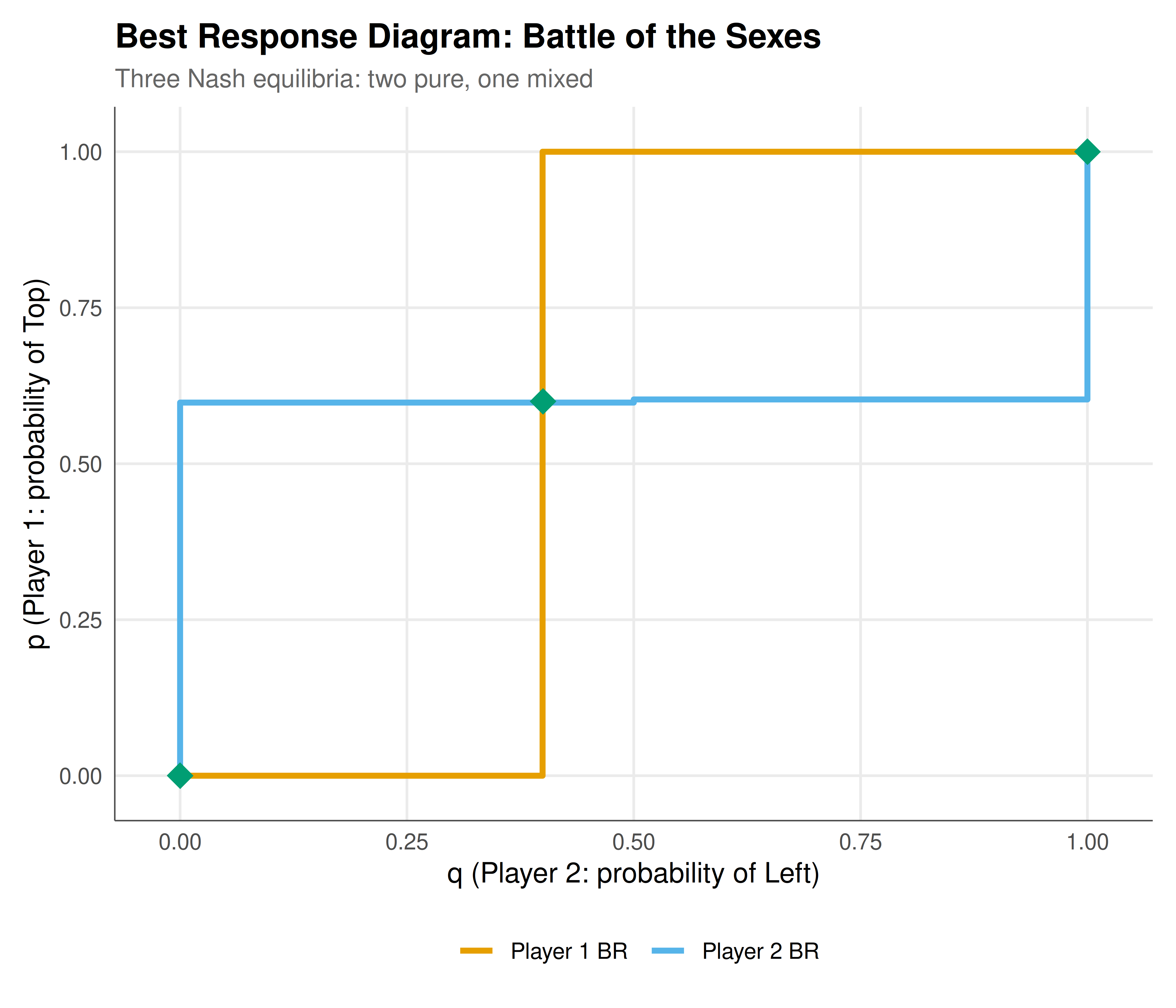
The figure below recreates what the 2x2 game solver Shiny app would display for the Battle of the Sexes game. The best response correspondences for both players are shown, with Nash equilibria marked as green diamonds. The Battle of the Sexes has three Nash equilibria: two in pure strategies and one in mixed strategies.
```{r}
#| label: fig-shiny-static
#| fig-cap: "Figure 1. Best response diagram for the Battle of the Sexes game. Orange: Player 1's best response (probability of Top as a function of Player 2's mixing probability q). Blue: Player 2's best response (probability of Left as a function of Player 1's mixing probability p). Green diamonds mark Nash equilibria: two pure-strategy NE at (1,1) and (0,0), and one mixed-strategy NE."
#| dev: [png, pdf]
#| fig-width: 7
#| fig-height: 6
#| dpi: 300
brs <- compute_best_responses(3, 0, 0, 2, 2, 0, 0, 3)
bos_game <- solve_2x2_game(3, 0, 0, 2, 2, 0, 0, 3)

ne_points <- data.frame(
  q = sapply(bos_game$equilibria, function(e) e$q),
  p = sapply(bos_game$equilibria, function(e) e$p),
  label = sapply(bos_game$equilibria, function(e) e$type)
)

p_br <- ggplot() +
  geom_step(data = brs$br1, aes(x = q, y = p_br, colour = "Player 1 BR"),
            linewidth = 1.2, direction = "mid") +
  geom_step(data = brs$br2, aes(x = q_br, y = p, colour = "Player 2 BR"),
            linewidth = 1.2, direction = "mid") +
  geom_point(data = ne_points, aes(x = q, y = p,
    text = paste0("NE: ", label, "\nq = ", round(q, 3), ", p = ", round(p, 3))),
    colour = okabe_ito[3], size = 5, shape = 18) +
  scale_colour_manual(values = c("Player 1 BR" = okabe_ito[1],
                                  "Player 2 BR" = okabe_ito[2]),
                      name = "") +
  labs(title = "Best Response Diagram: Battle of the Sexes",
       subtitle = "Three Nash equilibria: two pure, one mixed",
       x = "q (Player 2: probability of Left)",
       y = "p (Player 1: probability of Top)") +
  coord_cartesian(xlim = c(-0.02, 1.02), ylim = c(-0.02, 1.02)) +
  theme_publication()

p_br
```
## Interactive figure
Hover over the Nash equilibrium points to see the exact mixing probabilities. The interactive version allows you to zoom in on the mixed-strategy equilibrium, which is located in the interior of the strategy space.
```{r}
#| label: fig-shiny-interactive
# Cournot comparative statics - interactive
cournot_long <- cournot_data |>
  pivot_longer(cols = c(price, profit_i), names_to = "variable",
               values_to = "value") |>
  mutate(
    variable_label = ifelse(variable == "price", "Equilibrium Price",
                            "Profit per Firm"),
    text = paste0("Firms: ", n_firms,
                  "\n", variable_label, ": ", round(value, 2),
                  "\nq_i: ", round(q_i, 2),
                  "\nQ_total: ", round(Q_total, 2))
  )

p_cournot <- ggplot(cournot_long, aes(x = n_firms, y = value,
                                       colour = variable_label, text = text)) +
  geom_line(linewidth = 1) +
  geom_point(size = 2.5) +
  scale_colour_manual(values = c("Equilibrium Price" = okabe_ito[1],
                                  "Profit per Firm" = okabe_ito[2]),
                      name = "") +
  scale_x_continuous(breaks = 1:10) +
  labs(title = "Cournot Equilibrium: Price and Profit vs. Number of Firms",
       subtitle = "Parameters: a = 100, b = 1, c = 20",
       x = "Number of firms",
       y = "Value") +
  theme_publication()

ggplotly(p_cournot, tooltip = "text") |>
  config(displaylogo = FALSE,
         modeBarButtonsToRemove = c("select2d", "lasso2d"))
```
## Interpretation
The three Shiny apps presented in this tutorial serve different but complementary pedagogical and analytical purposes. The 2x2 game solver is perhaps the most immediately useful: it allows students and researchers to quickly classify any $2 \times 2$ game, find all Nash equilibria, and visualise the best response structure. The best response diagram is a powerful visual tool because it makes the logic of Nash equilibrium transparent. A Nash equilibrium is a point where both players are simultaneously best-responding to each other, which corresponds visually to an intersection of the two best response correspondences. By changing the payoff values, the user can explore how the number and location of equilibria change, providing intuition for concepts like the distinction between dominance-solvable games (where best responses are constant functions) and coordination games (where best responses create multiple intersections).
The Cournot duopoly simulator illustrates one of the most important results in industrial organisation: as the number of competing firms increases, the equilibrium price falls toward marginal cost and individual profits shrink toward zero. This is the Cournot convergence theorem, which establishes a smooth transition from monopoly (one firm, high price, high profit) to perfect competition (many firms, price equals marginal cost, zero economic profit). The interactive slider for the number of firms makes this convergence vivid. The app also shows how the best response functions shift when demand or cost parameters change, providing intuition for comparative statics. For example, increasing the demand intercept $a$ shifts both best response functions outward, increasing equilibrium quantities and profits. Increasing marginal cost $c$ shifts them inward. These relationships are immediate in the interactive app but require algebraic manipulation to derive from the formulas.
The evolutionary dynamics visualiser provides the richest visual experience. The phase portrait on the simplex shows the flow of the replicator dynamics for any $3 \times 3$ payoff matrix. Different payoff matrices produce qualitatively different phase portraits: Rock-Paper-Scissors produces closed orbits around the interior fixed point; a coordination game produces three basins of attraction, each leading to fixation of one strategy; a game with a single dominant strategy shows all trajectories converging to one vertex. The ability to switch between these cases with preset buttons and to modify individual payoff entries encourages systematic exploration of how payoff structure determines dynamics. The phase portrait also reveals features that are difficult to see in time-series plots, such as the shape of basins of attraction and the location of saddle points on the boundary of the simplex.
From a software engineering perspective, the separation of computation from presentation is a key design principle. The core functions --- `solve_2x2_game`, `cournot_equilibrium`, `replicator_euler` --- are pure functions that take inputs and return outputs without any Shiny-specific code. This separation has three benefits. First, the functions can be tested independently using unit tests. Second, they can be reused in other contexts, such as batch simulations or static reports. Third, the Shiny server code becomes a thin wrapper that calls the core functions and passes the results to the UI, making the app easier to maintain and extend. This architecture --- separating the "model" from the "view" --- is a standard best practice in software development that applies equally well to scientific computing.
These apps are starting points, not finished products. Natural extensions include adding quantal response equilibrium (QRE) computation to the game solver, implementing Stackelberg (sequential move) equilibria for the Cournot app, and adding mutation and selection intensity parameters to the evolutionary dynamics visualiser. The modular architecture of the code makes such extensions straightforward to implement.
## Extensions & related tutorials
- [Publication-ready ggplot themes](../../visualization-and-communication/publication-ready-ggplot-theme/) --- Advanced ggplot2 customisation for game theory visualisations, including the theme used in this tutorial.
- [Interactive game theory dashboards](../../visualization-and-communication/interactive-game-theory-dashboards/) --- Building more complex dashboards with multiple linked views using Shiny and plotly.
- [Battle of the Sexes](../../classical-games/battle-of-the-sexes/) --- Detailed analysis of the game used as the static figure example in this tutorial.
- [Replicator dynamics simulation](../../simulations/replicator-dynamics-simulation/) --- In-depth computational analysis of the replicator dynamics that powers App 3.
- [Expected utility foundations](../../decision-theory/expected-utility-foundations/) --- The decision-theoretic foundations underlying the payoff structures analysed in these apps.
## References
::: {#refs}
:::