40 Case Study 2: Institutional Benchmarking
40.1 Objective
Compare publication output, citation impact, and research profiles of five universities using size-independent and field-normalised indicators.
40.3 Data acquisition
institutions <- tribble(
  ~short_name,    ~oa_id,
  "MIT",          "I63966007",
  "Oxford",       "I40120149",
  "ETH Zurich",   "I202697423",
  "U São Paulo",  "I66491032",
  "U Cape Town",  "I173603587"
)
fetch_works <- function(inst_id) {
  res <- tryCatch(
    oa_fetch(
      entity = "works",
      authorships.institutions.id = inst_id,
      from_publication_date = "2020-01-01",
      to_publication_date = "2022-12-31",
      type = "article",
      options = list(sample = 300, seed = 42)
    ),
    error = function(e) NULL
  )
  if (is.null(res)) tibble() else res
}

inst_data <- institutions |>
  mutate(works = map(oa_id, fetch_works)) |>
  filter(map_int(works, nrow) > 0)
40.4 Publication volume
inst_data |>
  mutate(n = map_int(works, nrow)) |>
  ggplot(aes(x = n, y = reorder(short_name, n))) +
  geom_col(fill = palette_sci(1)) +
  labs(x = "Sampled articles", y = NULL) +
  theme_sci()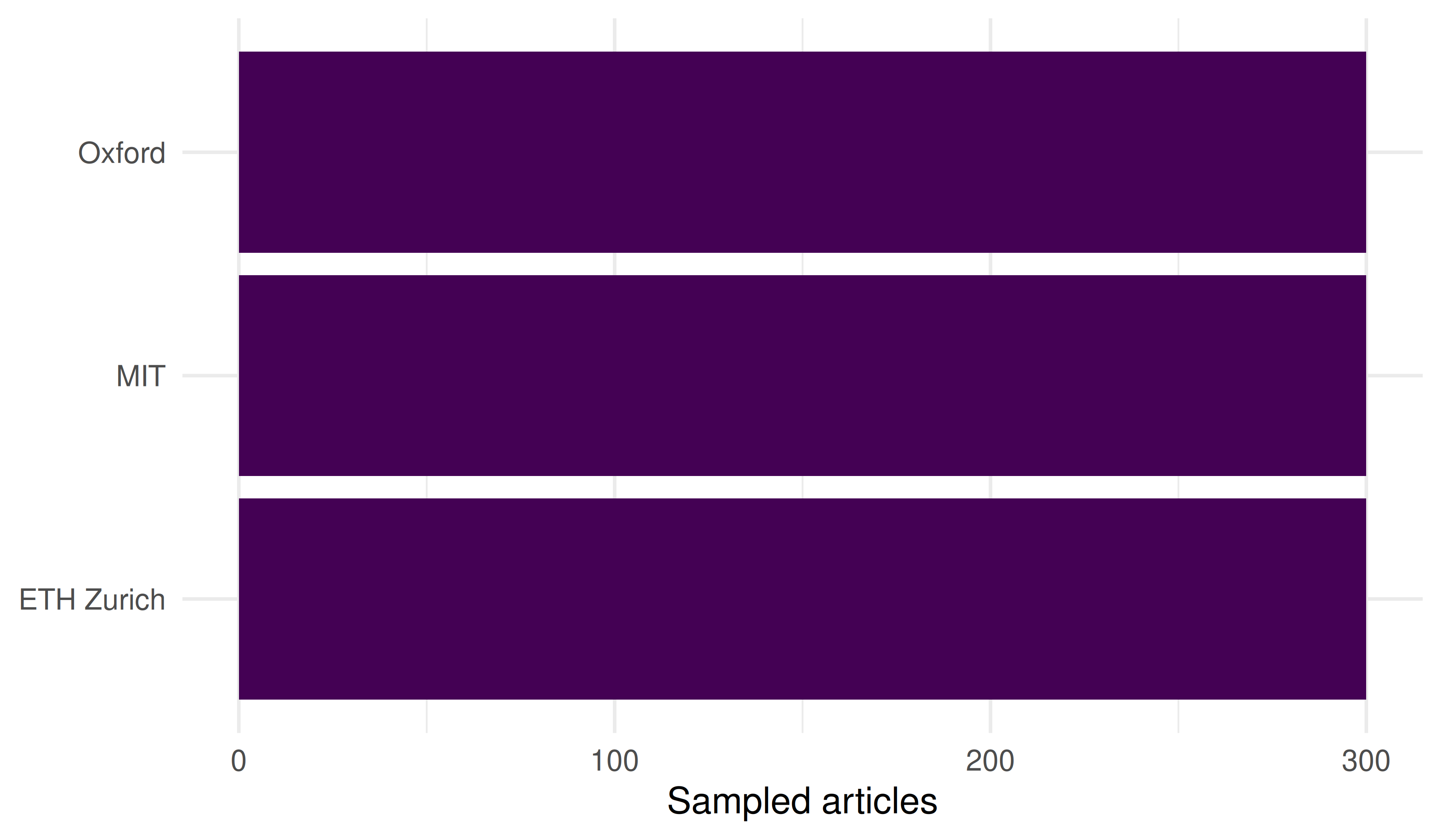
Figure 40.1: Sampled publication counts by institution.
40.5 Citation impact
impact <- inst_data |>
  mutate(
    mean_cites = map_dbl(works, \(w) mean(w$cited_by_count, na.rm = TRUE)),
    median_cites = map_dbl(works, \(w) median(w$cited_by_count, na.rm = TRUE)),
    h_index = map_int(works, \(w) compute_h_index(w$cited_by_count))
  ) |>
  select(short_name, mean_cites, median_cites, h_index) |>
  arrange(desc(mean_cites))

impact |>
  gt() |>
fmt_number(columns = mean_cites, decimals = 1)| short_name | mean_cites | median_cites | h_index |
|---|---|---|---|
| Oxford | 43.4 | 17.0 | 55 |
| MIT | 37.0 | 13.5 | 50 |
| ETH Zurich | 27.0 | 13.0 | 45 |
40.6 Full vs. fractional counting
counting <- inst_data |>
  mutate(
    full_count = map_int(works, nrow),
    frac_count = map_dbl(works, function(w) {
      w |>
        select(id, authorships) |>
        unnest(authorships, names_sep = "_") |>
        unnest(authorships_affiliations, names_sep = "_") |>
        group_by(id) |>
        summarise(n_inst = n_distinct(authorships_affiliations_id),
                  .groups = "drop") |>
        mutate(frac = 1 / pmax(n_inst, 1)) |>
        pull(frac) |>
        sum()
    })
  ) |>
  select(short_name, full_count, frac_count) |>
  mutate(ratio = round(frac_count / full_count, 2))

counting |> gt()| short_name | full_count | frac_count | ratio |
|---|---|---|---|
| MIT | 300 | 118 | 0.39 |
| Oxford | 300 | 101 | 0.34 |
| ETH Zurich | 300 | 110 | 0.37 |
counting |>
  pivot_longer(c(full_count, frac_count), names_to = "method", values_to = "count") |>
  mutate(method = recode(method, full_count = "Full", frac_count = "Fractional")) |>
  ggplot(aes(x = count, y = reorder(short_name, count), fill = method)) +
  geom_col(position = "dodge", width = 0.7) +
  scale_fill_manual(values = palette_sci(2)) +
  labs(x = "Count", y = NULL, fill = "Method") +
  theme_sci()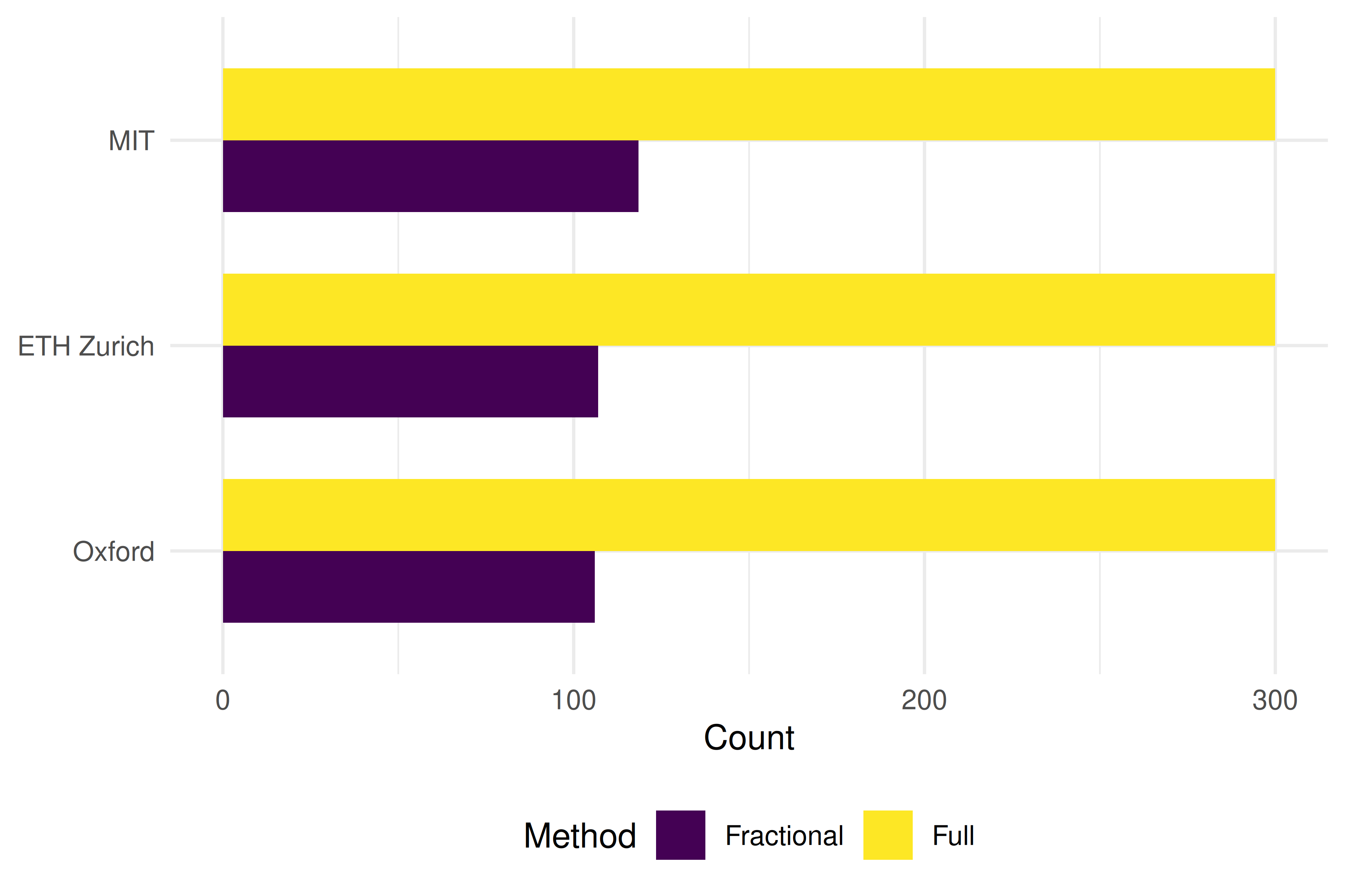
Figure 40.2: Full vs. fractional publication counts.
40.7 OA rates
inst_data |>
  mutate(oa_rate = map_dbl(works, \(w) mean(w$oa_status != "closed", na.rm = TRUE))) |>
  ggplot(aes(x = oa_rate, y = reorder(short_name, oa_rate))) +
  geom_col(fill = palette_sci(1)) +
  scale_x_continuous(labels = scales::percent) +
  labs(x = "OA rate", y = NULL) +
  theme_sci()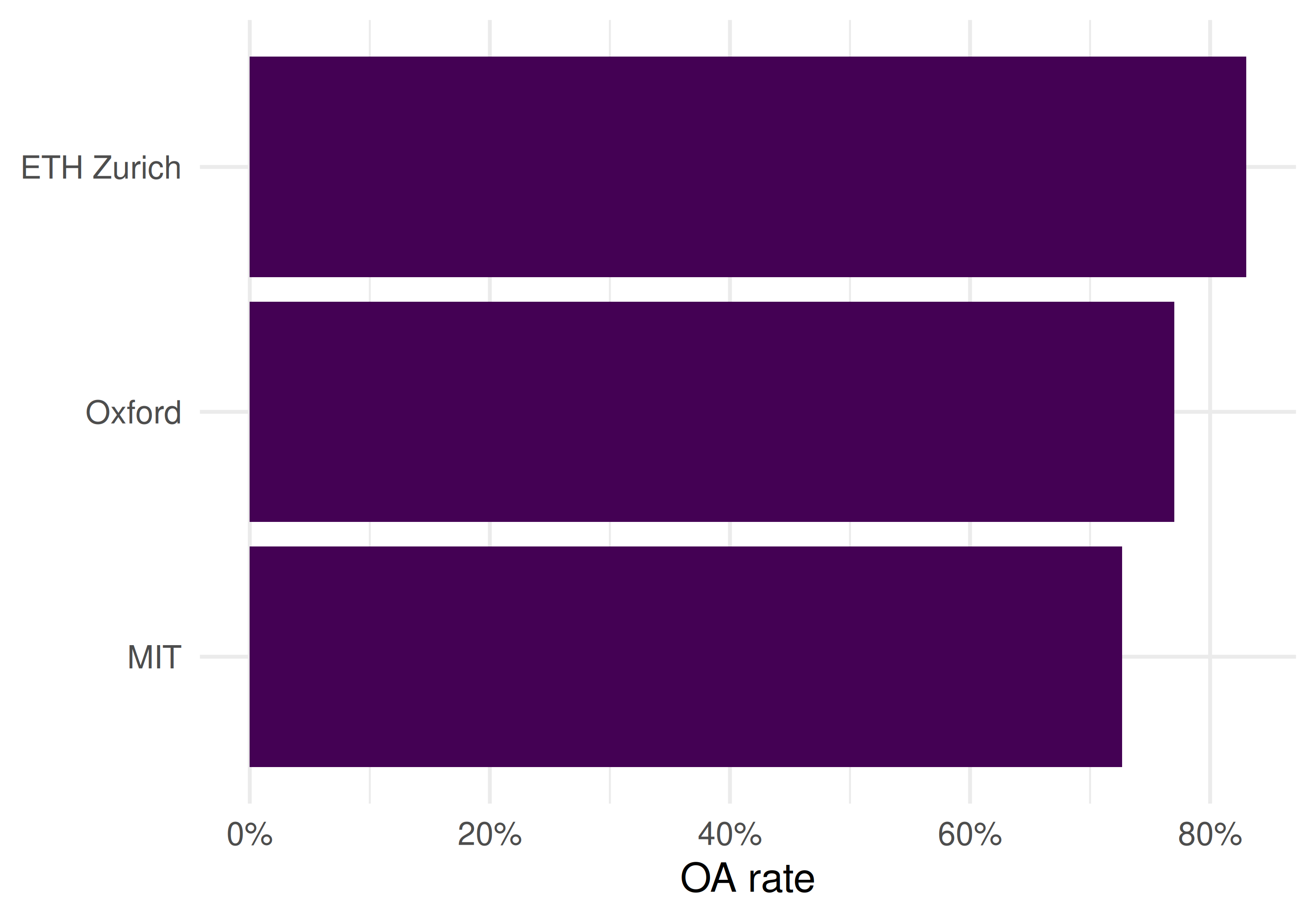
Figure 40.3: Open access rate by institution.
40.8 Key findings
- Size vs. impact: Raw publication counts favour larger institutions. Fractional counting and h-index provide size-independent comparisons.
- Collaboration intensity: Institutions with lower fractional/full ratios have more inter-institutional collaborations.
- OA variation: OA rates differ substantially, reflecting different national mandates and institutional policies.
- No single ranking: Different indicators produce different orderings. This illustrates the Leiden Manifesto principle that multiple indicators are needed for fair comparison (Hicks et al. 2015).
40.9 Lessons learned
- Sampling introduces uncertainty: these are illustrative comparisons, not definitive rankings.
- Field mix confounds all comparisons: a medical university and a technical university are not directly comparable without field normalisation.
- Responsible benchmarking requires reporting the counting method, normalisation approach, and sample size transparently.
This book was built by the bookdown R package.