42 Case Study 4: Gender Gap in Scientific Publishing

42.1 Objective

Compare gender representation in authorship across a biomedical journal and an information-science journal, demonstrating both the methods and their substantial limitations.

42.2 Setup

library(tidyverse)
library(openalexR)
library(glue)
library(gt)

set.seed(20260509)

source(here::here("R", "api_helpers.R"))
source(here::here("R", "utils.R"))
source(here::here("R", "sci_palette.R"))

42.3 Data acquisition

works_sciento <- oa_fetch(
  entity = "works",
  primary_location.source.id = "S148561398",
  from_publication_date = "2019-01-01",
  to_publication_date = "2023-12-31",
  type = "article",
  options = list(sample = 300, seed = 42)
) |> mutate(journal = "Scientometrics")

works_plos <- oa_fetch(
  entity = "works",
  primary_location.source.id = "S202381698",
  from_publication_date = "2019-01-01",
  to_publication_date = "2023-12-31",
  type = "article",
  options = list(sample = 300, seed = 42)
) |> mutate(journal = "PLOS ONE")

works_all <- bind_rows(works_sciento, works_plos)

42.4 Gender inference

common_female <- c("maria", "anna", "li", "sarah", "jennifer", "jessica",
                   "elena", "nina", "laura", "julia", "diana", "sandra",
                   "lisa", "emily", "rachel", "amy", "kate", "megan")
common_male <- c("john", "david", "michael", "james", "robert", "peter",
                 "mark", "thomas", "paul", "daniel", "andreas", "martin",
                 "chris", "matthew", "andrew", "william", "kevin", "brian")

authors <- works_all |>
  select(work_id = id, journal, authorships) |>
  unnest(authorships, names_sep = "_") |>
  group_by(work_id) |>
  mutate(
    n_authors = n(),
    position = case_when(
      row_number() == 1 ~ "first",
      row_number() == n() & n() > 1 ~ "last",
      TRUE ~ "middle"
    )
  ) |>
  ungroup() |>
  mutate(
    first_name = str_to_lower(str_extract(authorships_display_name, "^\\S+")),
    gender = case_when(
      first_name %in% common_female ~ "female",
      first_name %in% common_male ~ "male",
      TRUE ~ NA_character_
    )
  ) |>
  filter(!is.na(gender))

cat(glue("Classified authors: {nrow(authors)}\n"))

#> Classified authors: 221

42.5 Gender representation by journal

authors |>
  count(journal, gender) |>
  group_by(journal) |>
  mutate(pct = n / sum(n)) |>
  ggplot(aes(x = journal, y = pct, fill = gender)) +
  geom_col(position = "dodge") +
  scale_y_continuous(labels = scales::percent) +
  scale_fill_manual(values = palette_sci(2)) +
  labs(x = NULL, y = "Proportion", fill = "Gender") +
  theme_sci()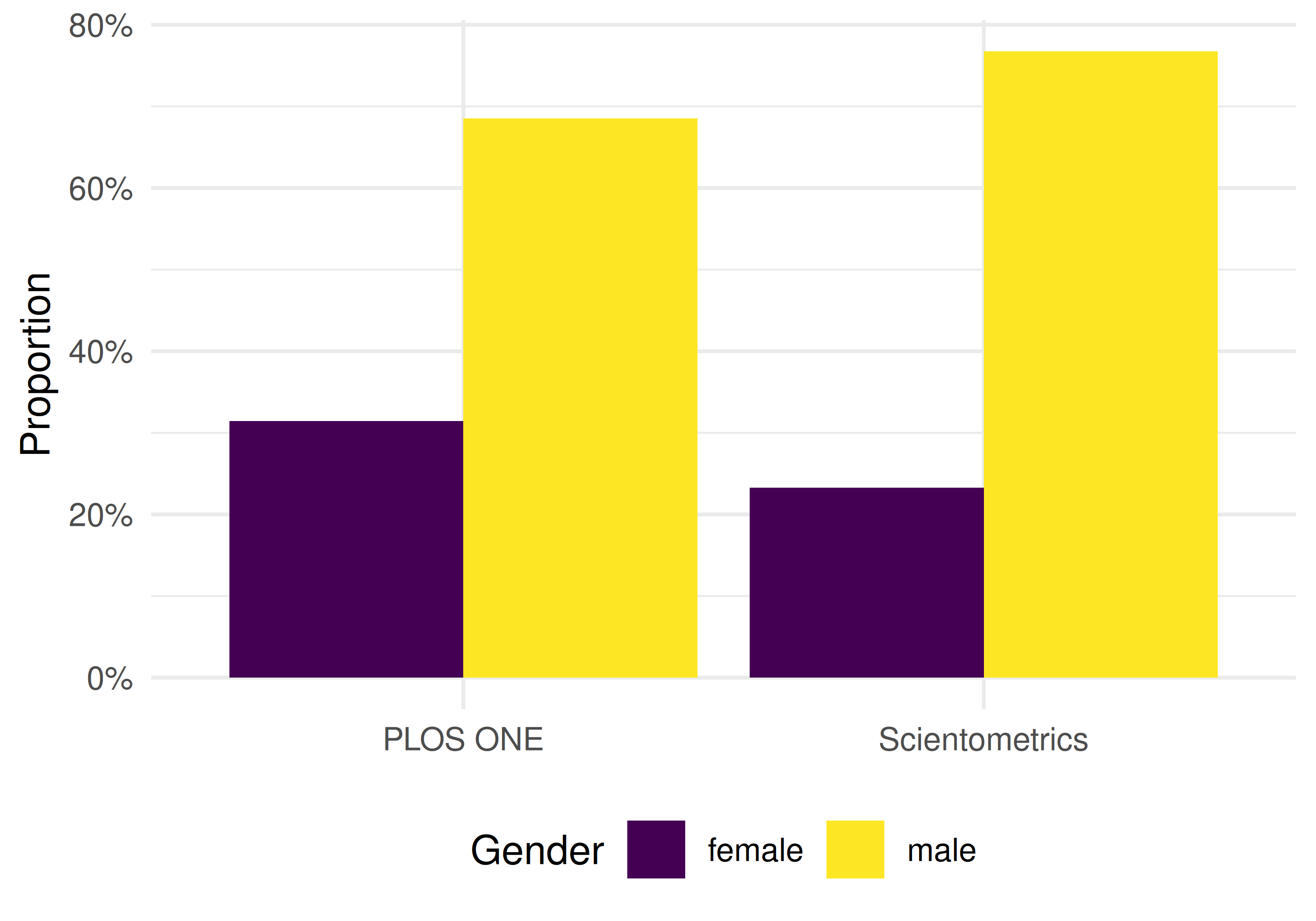

Figure 42.1: Gender representation by journal.

42.6 Authorship position analysis

position_summary <- authors |>
  count(journal, position, gender) |>
  group_by(journal, position) |>
  mutate(pct = n / sum(n)) |>
  ungroup()

ggplot(position_summary, aes(x = position, y = pct, fill = gender)) +
  geom_col(position = "dodge") +
  facet_wrap(~ journal) +
  scale_y_continuous(labels = scales::percent) +
  scale_fill_manual(values = palette_sci(2)) +
  labs(x = "Author position", y = "Proportion", fill = "Gender") +
  theme_sci()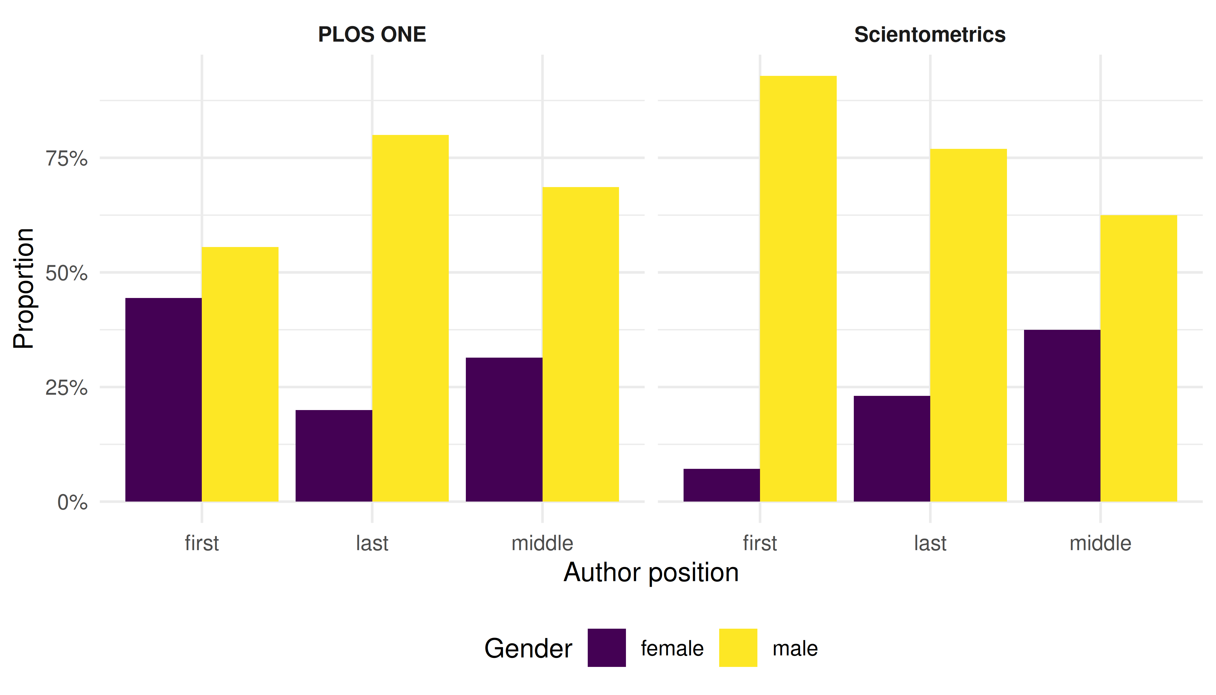

Figure 42.2: Gender representation by authorship position and journal.

42.7 Temporal trends

first_authors <- authors |>
  filter(position == "first") |>
  mutate(year = year(as.Date(paste0(
    str_extract(work_id, "\\d{4}$"), "-01-01"
  ))))

works_all_year <- works_all |>
  transmute(work_id = id, year = year(publication_date))

first_authors_year <- first_authors |>
  select(-year) |>
  left_join(works_all_year, by = "work_id")

first_authors_year |>
  group_by(journal, year) |>
  summarise(female_pct = mean(gender == "female"), .groups = "drop") |>
  ggplot(aes(x = year, y = female_pct, colour = journal)) +
  geom_line(linewidth = 1) +
  geom_point(size = 2) +
  scale_y_continuous(labels = scales::percent) +
  scale_colour_manual(values = palette_sci(2)) +
  labs(x = "Year", y = "Female first-author proportion", colour = "Journal") +
  theme_sci()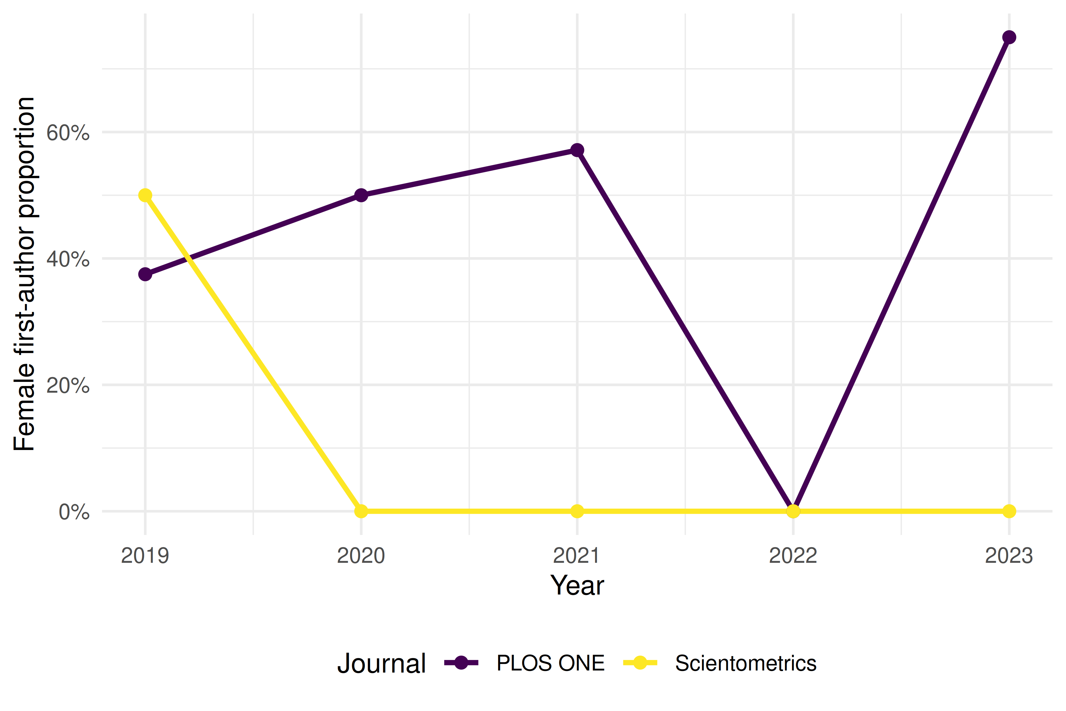

Figure 42.3: Proportion of female first authors by year.

42.8 Key findings

1. Persistent gap: Male names are overrepresented in both journals, particularly in last-author positions.
2. Disciplinary differences: The gender balance differs between journals, likely reflecting field-specific demographics.
3. Temporal progress: Some evidence of increasing female representation over time, but trends are noisy due to small sample sizes.

42.9 Critical caveats

These results must be interpreted with extreme caution:

• Name-based inference enforces a binary that excludes non-binary researchers.
• Coverage is biased: names from East Asia, South Asia, and Africa are poorly classified.
• The unclassified names are not random — they are systematically different from classified names.
• This is a methodological demonstration, not a definitive study. Production gender analysis requires validated tools with confidence scores and country context (Larivière et al. 2013).

This book was built by the bookdown R package.