17 Co-citation and Bibliographic Coupling
17.1 Learning objectives
After completing this chapter, you will be able to:
- Distinguish co-citation analysis from bibliographic coupling and explain when each is appropriate
- Construct co-citation and bibliographic coupling networks from OpenAlex reference data
- Compute normalised similarity measures (cosine, Jaccard) for citation-based linkages
- Identify core documents and intellectual clusters in a research field
- Interpret co-citation maps as representations of intellectual structure
17.3 Conceptual background
While co-authorship networks (16.3) reveal social structure, co-citation and bibliographic coupling networks reveal intellectual structure — the conceptual relationships between documents as expressed through citation behaviour.
Co-citation analysis, introduced independently by Small (1973) and Marshakova-Shaikevich in 1973, measures the relatedness of two documents by how often they are cited together by other papers. If documents A and B frequently appear in the same reference lists, they likely address related topics or represent complementary contributions to a field. Co-citation strength changes over time: as a field evolves, new citing papers create new co-citation links and strengthen or weaken existing ones.
Bibliographic coupling, proposed by Kessler (1963), takes the complementary perspective. Two documents are bibliographically coupled if they share one or more references. Unlike co-citation, coupling strength is fixed at publication time — once a paper is published, its reference list does not change. This makes bibliographic coupling especially useful for analysing the most recent literature, where co-citation links have not yet had time to form.
The two methods reveal different facets of intellectual structure. Co-citation maps the reception of ideas (how the community groups prior work); bibliographic coupling maps the production of knowledge (how authors draw on shared foundations). Waltman et al. (2010) demonstrated that combining both perspectives yields richer maps of science than either alone.
Both methods produce similarity matrices that can be converted to networks. Common normalisation approaches include cosine similarity (emphasising relative overlap) and the Jaccard index (penalising pairs with many unshared references). Unnormalised raw counts are dominated by highly-cited papers; normalisation is essential for balanced network construction.
17.4 Worked example
17.4.1 Fetching citing and cited works
We fetch a corpus of scientometrics research and extract reference lists.
works <- oa_fetch(
  entity = "works",
  primary_location.source.id = "S148561398",
  from_publication_date = "2020-01-01",
  to_publication_date = "2023-12-31",
  options = list(sample = 200, seed = 42)
)

refs <- works |>
  select(citing_id = id, referenced_works) |>
  unnest(referenced_works) |>
  rename(cited_id = referenced_works)

cat(glue("Citing works: {n_distinct(refs$citing_id)}\n"))
#> Citing works: 200#> Cited works: 8698#> Citation links: 994917.4.2 Building a co-citation network
Two cited documents are co-cited when they appear in the same reference list. We count shared citing papers.
cocit_pairs <- refs |>
  inner_join(refs, by = "citing_id", suffix = c("_a", "_b"),
             relationship = "many-to-many") |>
  filter(cited_id_a < cited_id_b) |>
  count(cited_id_a, cited_id_b, name = "cocit_count")

cocit_top <- cocit_pairs |>
  filter(cocit_count >= 3)

cat(glue("Co-citation pairs (count >= 3): {nrow(cocit_top)}\n"))
#> Co-citation pairs (count >= 3): 113
g_cocit <- graph_from_data_frame(
  cocit_top |> select(cited_id_a, cited_id_b, weight = cocit_count),
  directed = FALSE
) |>
  simplify(edge.attr.comb = list(weight = "sum"))

cat(glue("Co-citation network: {vcount(g_cocit)} nodes, {ecount(g_cocit)} edges\n"))
#> Co-citation network: 102 nodes, 113 edges17.4.3 Building a bibliographic coupling network
Two citing documents are coupled when they share at least one reference.
bibcoup_pairs <- refs |>
  inner_join(refs, by = "cited_id", suffix = c("_a", "_b"),
             relationship = "many-to-many") |>
  filter(citing_id_a < citing_id_b) |>
  count(citing_id_a, citing_id_b, name = "shared_refs")

bibcoup_top <- bibcoup_pairs |>
  filter(shared_refs >= 5)

cat(glue("Bibliographic coupling pairs (shared refs >= 5): {nrow(bibcoup_top)}\n"))
#> Bibliographic coupling pairs (shared refs >= 5): 48
g_bibcoup <- graph_from_data_frame(
  bibcoup_top |> select(citing_id_a, citing_id_b, weight = shared_refs),
  directed = FALSE
) |>
  simplify(edge.attr.comb = list(weight = "sum"))

cat(glue("Coupling network: {vcount(g_bibcoup)} nodes, {ecount(g_bibcoup)} edges\n"))
#> Coupling network: 62 nodes, 48 edges17.4.4 Visualisation
comp <- components(g_cocit)
giant <- induced_subgraph(g_cocit, which(comp$membership == which.max(comp$csize)))
V(giant)$community <- as.factor(membership(cluster_leiden(
  giant, resolution_parameter = 1.0, objective_function = "modularity"
)))
V(giant)$degree <- degree(giant)

set.seed(42)
layout <- create_layout(as_tbl_graph(giant), layout = "fr")

ggraph(layout) +
  geom_edge_link(alpha = 0.1, colour = "grey60") +
  geom_node_point(aes(size = degree, colour = community), alpha = 0.8) +
  scale_size_continuous(range = c(1, 5), guide = "none") +
  scale_colour_manual(values = palette_sci(
    n_distinct(V(giant)$community)
  )) +
  labs(colour = "Community") +
  theme_void(base_family = "sans", base_size = 11) +
  theme(legend.position = "bottom")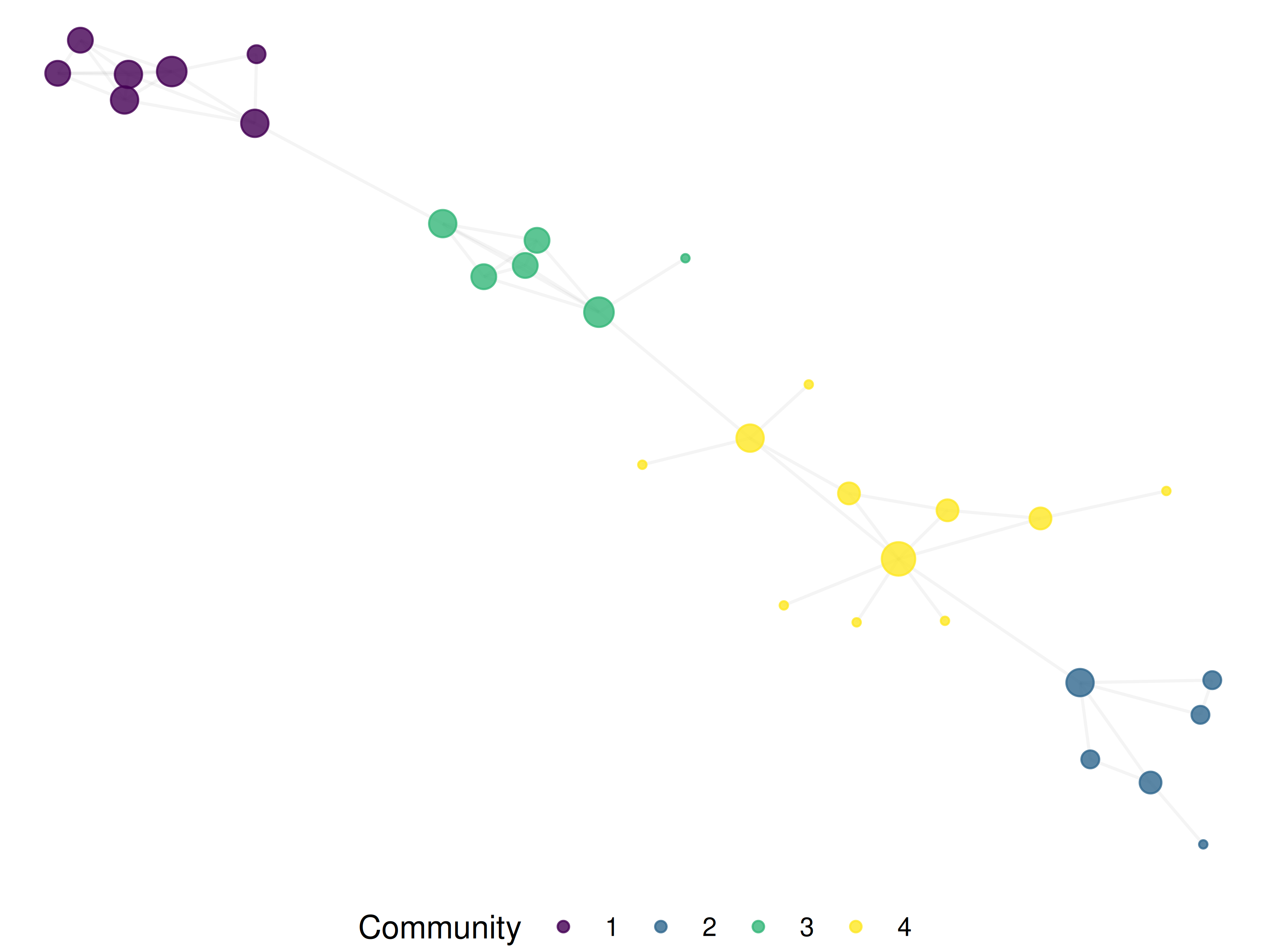
Figure 17.1: Co-citation network of frequently co-cited references in Scientometrics (2020–2023).
comp_bc <- components(g_bibcoup)
giant_bc <- induced_subgraph(g_bibcoup,
                             which(comp_bc$membership == which.max(comp_bc$csize)))
V(giant_bc)$community <- as.factor(membership(cluster_leiden(
  giant_bc, resolution_parameter = 1.0, objective_function = "modularity"
)))
V(giant_bc)$degree <- degree(giant_bc)

set.seed(42)
layout_bc <- create_layout(as_tbl_graph(giant_bc), layout = "fr")

ggraph(layout_bc) +
  geom_edge_link(alpha = 0.1, colour = "grey60") +
  geom_node_point(aes(size = degree, colour = community), alpha = 0.8) +
  scale_size_continuous(range = c(1, 5), guide = "none") +
  scale_colour_manual(values = palette_sci(
    n_distinct(V(giant_bc)$community)
  )) +
  labs(colour = "Community") +
  theme_void(base_family = "sans", base_size = 11) +
  theme(legend.position = "bottom")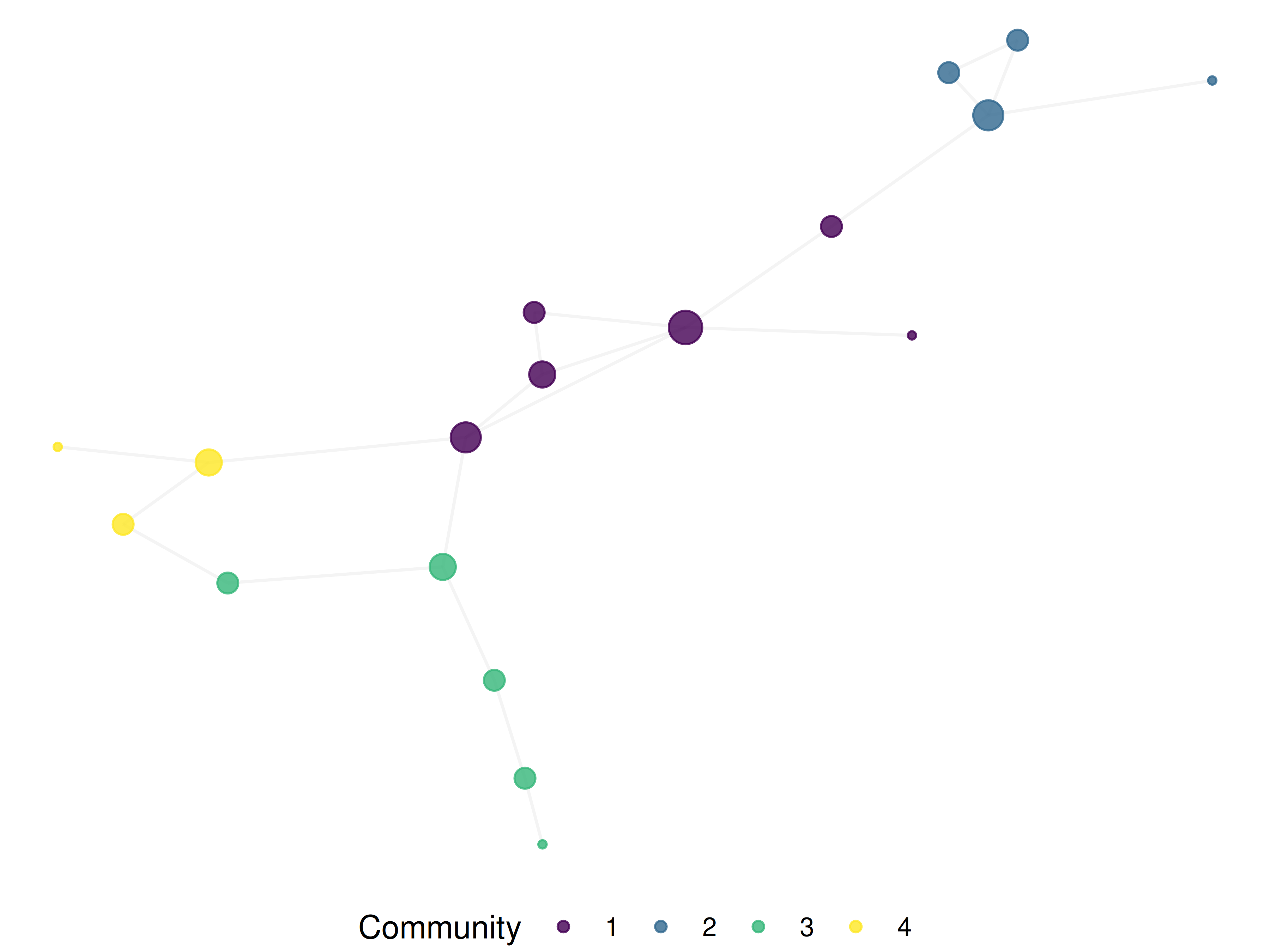
Figure 17.2: Bibliographic coupling network of Scientometrics articles (2020–2023).
17.4.5 Comparing the two approaches
comparison <- tibble(
  Method = c("Co-citation", "Bibliographic coupling"),
  Nodes = c(vcount(g_cocit), vcount(g_bibcoup)),
  Edges = c(ecount(g_cocit), ecount(g_bibcoup)),
  Components = c(components(g_cocit)$no, components(g_bibcoup)$no),
  Density = c(round(graph.density(g_cocit), 4),
              round(graph.density(g_bibcoup), 4))
)

comparison |> gt()| Method | Nodes | Edges | Components | Density |
|---|---|---|---|---|
| Co-citation | 102 | 113 | 28 | 0.0219 |
| Bibliographic coupling | 62 | 48 | 20 | 0.0254 |
17.5 Diagnostics and interpretation
- Threshold selection: The minimum co-citation count or shared-reference count determines network density. Too low a threshold creates a hairball; too high excludes important links. Experiment with multiple thresholds and report the chosen value.
- Normalisation: Raw co-citation counts favour highly cited papers. Cosine normalisation produces more balanced networks. Always report whether counts are raw or normalised.
- Giant component ratio: A fragmented co-citation network may indicate that the corpus spans multiple disconnected subfields, or that the threshold is too high.
- Temporal stability: Co-citation networks change as new papers cite old ones. Bibliographic coupling networks are fixed at publication time. If you need a stable snapshot of recent literature, coupling is preferable.
17.7 Limitations and responsible use
- Co-citation reflects citing behaviour, not truth. Frequently co-cited papers may be co-cited because they represent a dominant paradigm, not because they are the best or most relevant works. Minority viewpoints may be invisible.
- Reference list quality. Both methods depend entirely on the accuracy and completeness of reference lists. Missing references, formatting errors, and DOI mismatches reduce coverage. OpenAlex reference parsing is imperfect (Priem et al. 2022).
- Size effects. Papers with long reference lists contribute disproportionately to bibliographic coupling. Consider normalising by reference list length.
- Not evaluative. Co-citation and coupling measure relatedness, not quality. A highly co-cited paper is intellectually central, which is not the same as excellent or correct (Hicks et al. 2015).
17.9 Common pitfalls
- Confusing the two methods. Co-citation links cited documents; bibliographic coupling links citing documents. They answer different questions about the same citation data.
- Skipping normalisation. Raw counts produce networks dominated by a few highly cited papers. Always normalise for balanced analysis.
- Ignoring the threshold. Reporting results without specifying the minimum count or similarity cutoff makes the analysis irreproducible.
- Treating coupling as dynamic. Bibliographic coupling strength is fixed at publication. Do not interpret changes in coupling networks over time as evolving relationships — they reflect changes in the corpus, not the links.
17.10 Exercises
Cosine normalisation. Compute cosine-normalised co-citation strengths instead of raw counts. How does the network structure change? Do the same core documents emerge?
Temporal co-citation. Split the corpus into two time periods (2020–2021 and 2022–2023). Build a co-citation network for each. Which co-citation pairs are stable across periods, and which are new?
Bibliographic coupling by year. For each publication year, build a bibliographic coupling network and report the number of components and modularity. Does the intellectual structure become more or less fragmented over time?
Identifying research fronts. Use bibliographic coupling communities to identify research fronts. For each community, list the three most frequent keywords or title words. Do the fronts correspond to recognisable subfields?
17.11 Solutions
Solutions are provided in 2.11.
17.12 Further reading
- Small (1973) — Co-citation analysis: the foundational paper.
- Kessler (1963) — Bibliographic coupling: the original proposal.
- Waltman et al. (2010) — Unified approach to bibliometric network construction and clustering.
- Fortunato (2010) — Community detection methods applicable to citation networks.
- Garfield (1955) — The intellectual origins of citation indexing.
17.13 Session info
#> R version 4.4.1 (2024-06-14)
#> Platform: x86_64-pc-linux-gnu
#> Running under: Ubuntu 24.04.4 LTS
#>
#> Matrix products: default
#> BLAS:   /usr/lib/x86_64-linux-gnu/openblas-pthread/libblas.so.3
#> LAPACK: /usr/lib/x86_64-linux-gnu/openblas-pthread/libopenblasp-r0.3.26.so;  LAPACK version 3.12.0
#>
#> locale:
#>  [1] LC_CTYPE=C.UTF-8       LC_NUMERIC=C           LC_TIME=C.UTF-8
#>  [4] LC_COLLATE=C.UTF-8     LC_MONETARY=C.UTF-8    LC_MESSAGES=C.UTF-8
#>  [7] LC_PAPER=C.UTF-8       LC_NAME=C              LC_ADDRESS=C
#> [10] LC_TELEPHONE=C         LC_MEASUREMENT=C.UTF-8 LC_IDENTIFICATION=C
#>
#> time zone: UTC
#> tzcode source: system (glibc)
#>
#> attached base packages:
#> [1] stats     graphics  grDevices utils     datasets  methods   base
#>
#> other attached packages:
#>  [1] ggraph_2.2.2       tidygraph_1.3.1    igraph_2.3.2       quanteda_4.4
#>  [5] pdftools_3.9.0     arrow_24.0.0       bibliometrix_5.4.0 RefManageR_1.4.0
#>  [9] bib2df_1.1.2.0     rcrossref_1.2.1    gt_1.3.0           tidytext_0.4.3
#> [13] glue_1.8.1         openalexR_3.0.1    lubridate_1.9.5    forcats_1.0.1
#> [17] stringr_1.6.0      dplyr_1.2.1        purrr_1.2.2        readr_2.2.0
#> [21] tidyr_1.3.2        tibble_3.3.1       ggplot2_4.0.3      tidyverse_2.0.0
#>
#> loaded via a namespace (and not attached):
#>   [1] bibtex_0.5.2           RColorBrewer_1.1-3     rstudioapi_0.18.0
#>   [4] jsonlite_2.0.0         magrittr_2.0.5         farver_2.1.2
#>   [7] rmarkdown_2.31         fs_2.1.0               vctrs_0.7.3
#>  [10] memoise_2.0.1          askpass_1.2.1          base64enc_0.1-6
#>  [13] htmltools_0.5.9        contentanalysis_1.0.0  curl_7.1.0
#>  [16] janeaustenr_1.0.0      cellranger_1.1.0       sass_0.4.10
#>  [19] bslib_0.11.0           htmlwidgets_1.6.4      tokenizers_0.3.0
#>  [22] plyr_1.8.9             httr2_1.2.2            plotly_4.12.0
#>  [25] cachem_1.1.0           dimensionsR_0.0.3      mime_0.13
#>  [28] lifecycle_1.0.5        pkgconfig_2.0.3        Matrix_1.7-0
#>  [31] R6_2.6.1               fastmap_1.2.0          shiny_1.13.0
#>  [34] digest_0.6.39          shinycssloaders_1.1.0  rprojroot_2.1.1
#>  [37] SnowballC_0.7.1        labeling_0.4.3         urltools_1.7.3.1
#>  [40] timechange_0.4.0       polyclip_1.10-7        httr_1.4.8
#>  [43] compiler_4.4.1         here_1.0.2             bit64_4.8.0
#>  [46] withr_3.0.2            S7_0.2.2               backports_1.5.1
#>  [49] viridis_0.6.5          ggforce_0.5.0          MASS_7.3-60.2
#>  [52] rappdirs_0.3.4         bibliometrixData_0.3.0 tools_4.4.1
#>  [55] otel_0.2.0             stopwords_2.3          zip_2.3.3
#>  [58] httpuv_1.6.17          rentrez_1.2.4          promises_1.5.0
#>  [61] grid_4.4.1             stringdist_0.9.17      generics_0.1.4
#>  [64] gtable_0.3.6           tzdb_0.5.0             rscopus_0.9.0
#>  [67] ca_0.71.1              data.table_1.18.4      hms_1.1.4
#>  [70] xml2_1.5.2             utf8_1.2.6             ggrepel_0.9.8
#>  [73] pillar_1.11.1          later_1.4.8            tweenr_2.0.3
#>  [76] brand.yml_0.1.0        lattice_0.22-6         bit_4.6.0
#>  [79] tidyselect_1.2.1       miniUI_0.1.2           downlit_0.4.5
#>  [82] knitr_1.51             gridExtra_2.3          bookdown_0.46
#>  [85] crul_1.6.0             xfun_0.57              graphlayouts_1.2.3
#>  [88] DT_0.34.0              humaniformat_0.6.0     visNetwork_2.1.4
#>  [91] stringi_1.8.7          lazyeval_0.2.3         qpdf_1.4.1
#>  [94] yaml_2.3.12            evaluate_1.0.5         codetools_0.2-20
#>  [97] httpcode_0.3.0         cli_3.6.6              xtable_1.8-8
#> [100] jquerylib_0.1.4        dichromat_2.0-0.1      Rcpp_1.1.1-1.1
#> [103] readxl_1.4.5           triebeard_0.4.1        XML_3.99-0.23
#> [106] parallel_4.4.1         assertthat_0.2.1       pubmedR_1.0.2
#> [109] viridisLite_0.4.3      scales_1.4.0           openxlsx_4.2.8.1
#> [112] rlang_1.2.0            fastmatch_1.1-8