23 Topic Modeling
23.1 Learning objectives
After completing this chapter, you will be able to:
- Explain the generative assumptions of LDA and STM
- Prepare a document-feature matrix suitable for topic modelling
- Fit LDA and STM models and select the number of topics
- Evaluate topic quality using coherence and exclusivity metrics
- Interpret and label topics using top words and representative documents
23.3 Conceptual background
A topic model is an unsupervised statistical model that discovers latent themes (topics) in a collection of documents. Each topic is a probability distribution over words; each document is a mixture of topics. The model “reverse-engineers” the writing process: given only the observed word frequencies, it infers which topics exist and how they are distributed across documents.
Latent Dirichlet Allocation (LDA) (Blei et al. 2003) is the foundational topic model. It assumes a generative process: for each document, draw a topic mixture from a Dirichlet prior; for each word position, draw a topic from that mixture, then draw a word from the topic’s word distribution. Inference (fitting the model) recovers the topic-word and document-topic distributions that best explain the observed data.
The Structural Topic Model (STM) (Roberts et al. 2019) extends LDA by allowing document-level covariates (e.g., publication year, journal) to influence topic prevalence and word usage. This is valuable for bibliometrics because we expect topics to vary systematically with time, discipline, and publication venue. STM also estimates a “content” component that lets word usage within a topic vary by covariate.
Choosing the number of topics (K) is the most consequential modelling decision. Too few topics produce overly broad themes; too many fragment coherent themes into noise. Quantitative approaches include held-out log-likelihood, semantic coherence, and exclusivity metrics. In practice, running models at multiple K values and inspecting the resulting topics is essential.
Topic models have been widely used in scientometrics to map research fields, track thematic evolution, identify emerging areas, and compare the topical focus of journals, institutions, or countries.
23.4 Worked example
23.4.1 Preparing the corpus
works <- oa_fetch(
  entity = "works",
  primary_location.source.id = "S148561398",
  from_publication_date = "2018-01-01",
  to_publication_date = "2023-12-31",
  options = list(sample = 400, seed = 42)
)

text_df <- works |>
  filter(!is.na(abstract), nchar(abstract) > 100) |>
  transmute(
    doc_id = id,
    text = paste(display_name, abstract, sep = ". "),
    year = year(publication_date)
  )

cat(glue("Documents for topic modelling: {nrow(text_df)}\n"))
#> Documents for topic modelling: 92
corp <- corpus(text_df, docid_field = "doc_id", text_field = "text")
docvars(corp, "year") <- text_df$year

toks <- tokens(corp, remove_punct = TRUE, remove_numbers = TRUE) |>
  tokens_tolower() |>
  tokens_remove(stopwords("en")) |>
  tokens_remove(c("study", "paper", "results", "research", "analysis",
                   "also", "however", "using", "based"))

dfmat <- dfm(toks) |>
  dfm_trim(min_termfreq = 5, min_docfreq = 3)

cat(glue("DFM: {nrow(dfmat)} docs x {ncol(dfmat)} features\n"))
#> DFM: 92 docs x 553 features23.4.2 Fitting LDA
dtm <- quanteda::convert(dfmat, to = "topicmodels")

lda_model <- LDA(dtm, k = 8, control = list(seed = 42))

lda_topics <- tidy(lda_model, matrix = "beta") |>
  rename(topic = topic, term = term, beta = beta)

cat(glue("LDA fitted with K = 8 topics\n"))
#> LDA fitted with K = 8 topics
lda_top_terms <- lda_topics |>
  group_by(topic) |>
  slice_max(beta, n = 10) |>
  ungroup() |>
  mutate(term = reorder_within(term, beta, topic))

ggplot(lda_top_terms, aes(x = beta, y = term, fill = factor(topic))) +
  geom_col(show.legend = FALSE) +
  facet_wrap(~ paste("Topic", topic), scales = "free_y", ncol = 4) +
  scale_y_reordered() +
  scale_fill_manual(values = palette_sci(8)) +
  labs(x = "Word probability (beta)", y = NULL) +
  theme_sci(base_size = 9)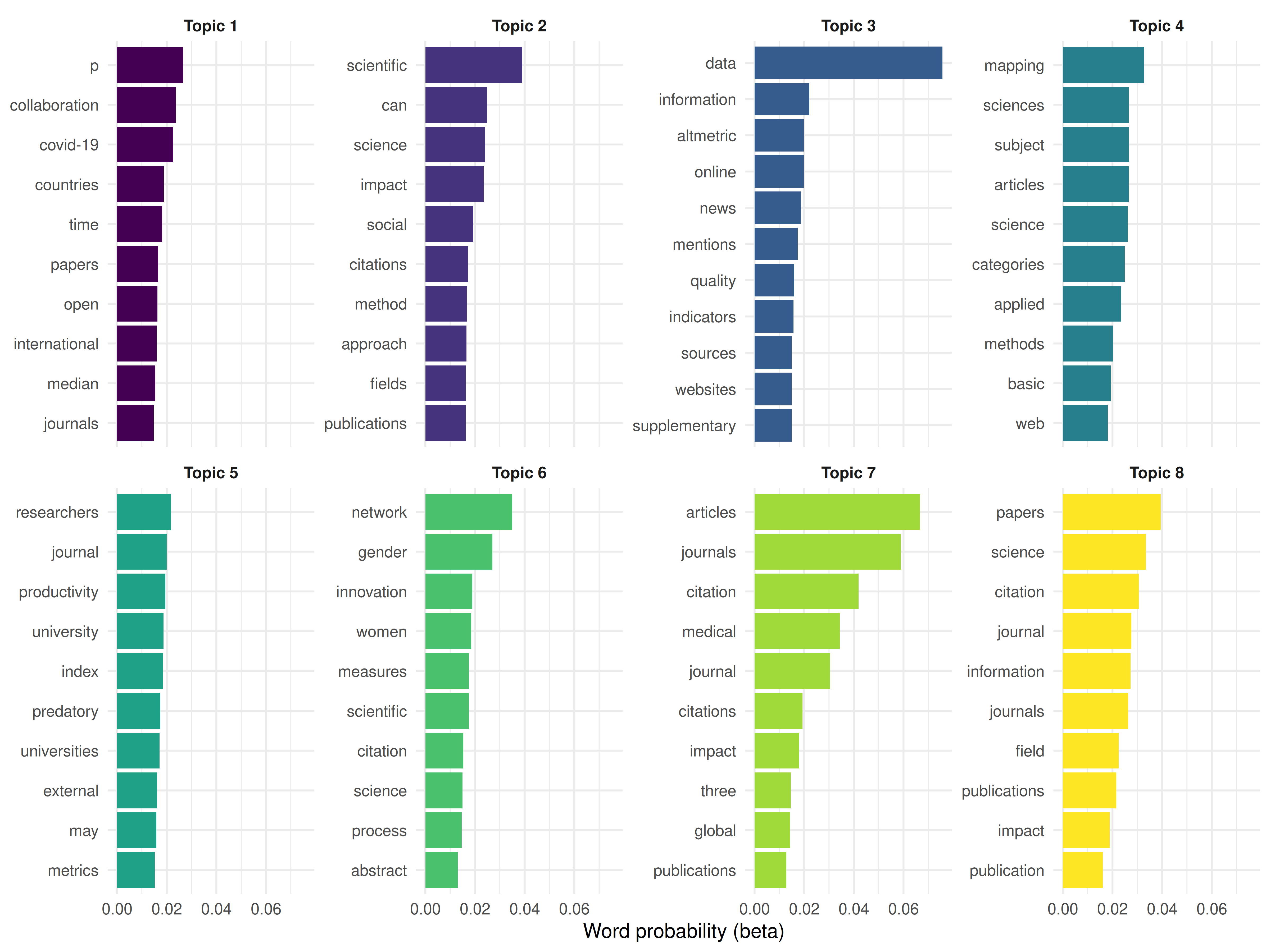
Figure 23.1: Top 10 terms per LDA topic.
23.4.3 Fitting STM with year covariate
stm_dfm <- quanteda::convert(dfmat, to = "stm")

stm_model <- stm(
  documents = stm_dfm$documents,
  vocab = stm_dfm$vocab,
  K = 8,
  prevalence = ~ year,
  data = stm_dfm$meta,
  seed = 42,
  verbose = FALSE
)

cat(glue("STM fitted with K = 8 topics, year as prevalence covariate\n"))
#> STM fitted with K = 8 topics, year as prevalence covariate
plot(stm_model, type = "summary", n = 5,
     main = "STM Topic Proportions and Top FREX Terms")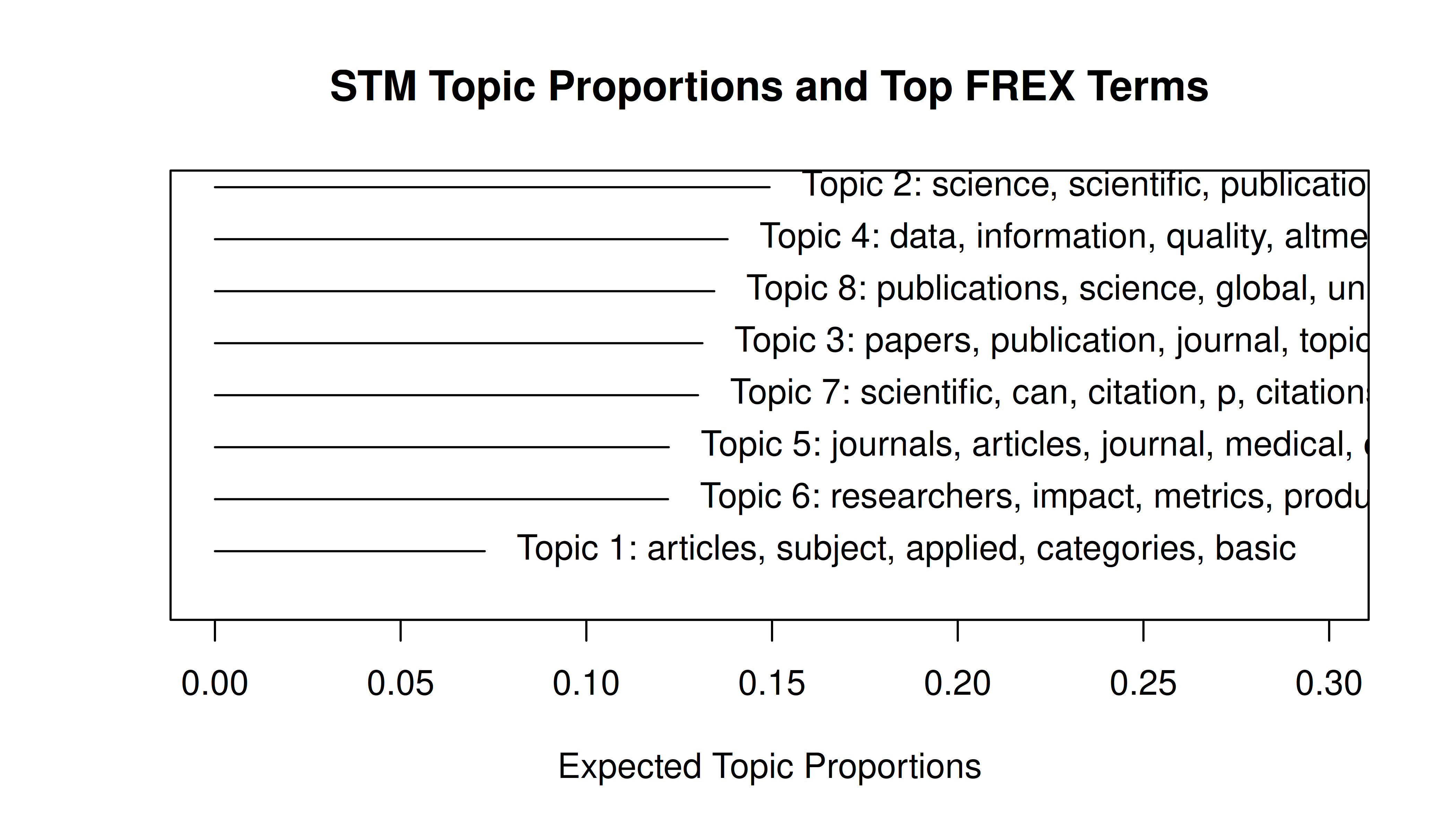
Figure 23.2: Top terms per STM topic, showing FREX (frequent and exclusive) words.
23.4.4 Topic prevalence over time
effect <- estimateEffect(1:8 ~ year, stm_model, meta = stm_dfm$meta)

effect_df <- map_dfr(1:8, function(k) {
  eff <- summary(effect, topics = k)$tables[[1]]
  tibble(
    topic = k,
    term = c("intercept", "year"),
    estimate = eff[, "Estimate"],
    se = eff[, "Std. Error"]
  )
}) |>
  filter(term == "year")

ggplot(effect_df, aes(x = factor(topic), y = estimate)) +
  geom_col(fill = palette_sci(1)) +
  geom_errorbar(aes(ymin = estimate - 1.96 * se, ymax = estimate + 1.96 * se),
                width = 0.3) +
  geom_hline(yintercept = 0, linetype = "dashed", colour = "grey50") +
  labs(x = "Topic", y = "Year effect on prevalence") +
  theme_sci()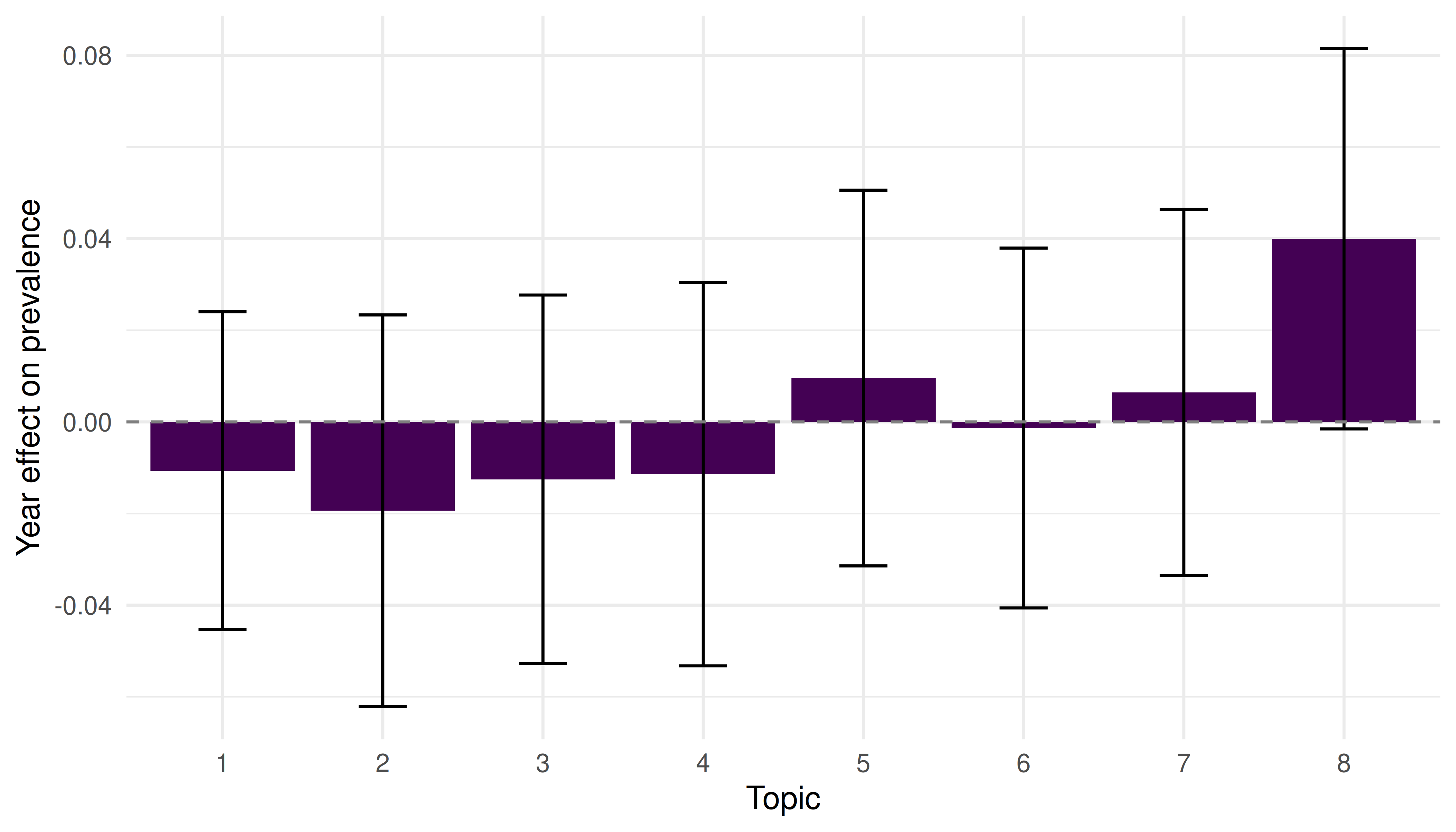
Figure 23.3: Estimated topic prevalence by publication year (STM).
23.4.5 Model diagnostics
coherence <- semanticCoherence(stm_model, stm_dfm$documents)
exclusivity <- exclusivity(stm_model)

diag_df <- tibble(
  topic = 1:8,
  coherence = round(coherence, 2),
  exclusivity = round(exclusivity, 2)
)

diag_df |> gt()| topic | coherence | exclusivity |
|---|---|---|
| 1 | -99.2 | 9.24 |
| 2 | -64.1 | 8.96 |
| 3 | -108.8 | 9.36 |
| 4 | -57.4 | 9.21 |
| 5 | -100.2 | 9.31 |
| 6 | -94.0 | 9.21 |
| 7 | -74.7 | 9.44 |
| 8 | -108.7 | 9.29 |
23.5 Diagnostics and interpretation
- Coherence: High coherence means the top words in a topic tend to co-occur in the same documents. Low coherence indicates a “junk” topic mixing unrelated terms.
- Exclusivity: High exclusivity means the top words are distinctive to that topic. Topics with low exclusivity share vocabulary with other topics, suggesting they may need to be split.
- Coherence-exclusivity trade-off: Adding more topics generally improves exclusivity but may decrease coherence. Plot both metrics across K values to find a balance.
- Human validation: Always read sample documents assigned to each topic. If a topic cannot be labelled by a domain expert, it may not represent a meaningful theme.
23.7 Limitations and responsible use
- Topics are not ground truth. Topic models are statistical constructs, not natural categories. Different random seeds, preprocessing choices, or K values produce different topics. Never claim a topic model reveals “the” structure of a field.
- Abstract-only models miss depth. Abstracts are compressed summaries. Topics derived from abstracts are coarser than those from full text.
- Number of topics is a researcher choice. There is no objectively correct K. Sensitivity analysis across multiple K values is essential.
- Temporal confounds. In STM, a topic that “grows” over time may reflect genuine intellectual shift or simply increased coverage by the database in recent years (Priem et al. 2022).
- Replication. Topic models are sensitive to preprocessing and random initialisation. Report all parameters and fix seeds for reproducibility.
23.9 Common pitfalls
- Not preprocessing enough. Rare terms, numbers, and generic academic vocabulary produce noisy topics. Trim the DFM before fitting.
- Choosing K by perplexity alone. Held-out perplexity often favours large K values that produce uninterpretable topics. Use coherence and exclusivity alongside perplexity.
- Treating topic proportions as precise measurements. Document-topic proportions are probabilistic estimates with uncertainty. Do not report them to three decimal places.
- Comparing topics across models. LDA and STM may number and define topics differently. Align topics by content, not by index.
23.10 Exercises
K selection. Fit LDA models with K = 5, 8, 12, and 15. Compute coherence for each. Plot coherence against K and select the best value. How sensitive are the results?
STM with journal covariate. Fetch data from two different journals. Fit an STM with journal as a prevalence covariate. Which topics differ most between journals?
Topic labelling. For the best LDA model, read the titles of the 5 documents with the highest proportion for each topic. Assign a human-readable label to each topic.
LDA vs. STM comparison. Compare the topics from LDA and STM for the same K. Are they similar? What does the STM’s year covariate add?
23.11 Solutions
Solutions are provided in 2.11.
23.13 Session info
#> R version 4.4.1 (2024-06-14)
#> Platform: x86_64-pc-linux-gnu
#> Running under: Ubuntu 24.04.4 LTS
#>
#> Matrix products: default
#> BLAS:   /usr/lib/x86_64-linux-gnu/openblas-pthread/libblas.so.3
#> LAPACK: /usr/lib/x86_64-linux-gnu/openblas-pthread/libopenblasp-r0.3.26.so;  LAPACK version 3.12.0
#>
#> locale:
#>  [1] LC_CTYPE=C.UTF-8       LC_NUMERIC=C           LC_TIME=C.UTF-8
#>  [4] LC_COLLATE=C.UTF-8     LC_MONETARY=C.UTF-8    LC_MESSAGES=C.UTF-8
#>  [7] LC_PAPER=C.UTF-8       LC_NAME=C              LC_ADDRESS=C
#> [10] LC_TELEPHONE=C         LC_MEASUREMENT=C.UTF-8 LC_IDENTIFICATION=C
#>
#> time zone: UTC
#> tzcode source: system (glibc)
#>
#> attached base packages:
#> [1] stats     graphics  grDevices utils     datasets  methods   base
#>
#> other attached packages:
#>  [1] stm_1.3.8                 topicmodels_0.2-17
#>  [3] quanteda.textstats_0.97.2 visNetwork_2.1.4
#>  [5] ggraph_2.2.2              tidygraph_1.3.1
#>  [7] igraph_2.3.2              quanteda_4.4
#>  [9] pdftools_3.9.0            arrow_24.0.0
#> [11] bibliometrix_5.4.0        RefManageR_1.4.0
#> [13] bib2df_1.1.2.0            rcrossref_1.2.1
#> [15] gt_1.3.0                  tidytext_0.4.3
#> [17] glue_1.8.1                openalexR_3.0.1
#> [19] lubridate_1.9.5           forcats_1.0.1
#> [21] stringr_1.6.0             dplyr_1.2.1
#> [23] purrr_1.2.2               readr_2.2.0
#> [25] tidyr_1.3.2               tibble_3.3.1
#> [27] ggplot2_4.0.3             tidyverse_2.0.0
#>
#> loaded via a namespace (and not attached):
#>   [1] bibtex_0.5.2           RColorBrewer_1.1-3     rstudioapi_0.18.0
#>   [4] jsonlite_2.0.0         magrittr_2.0.5         modeltools_0.2-24
#>   [7] farver_2.1.2           rmarkdown_2.31         fs_2.1.0
#>  [10] vctrs_0.7.3            memoise_2.0.1          askpass_1.2.1
#>  [13] base64enc_0.1-6        htmltools_0.5.9        contentanalysis_1.0.0
#>  [16] curl_7.1.0             janeaustenr_1.0.0      cellranger_1.1.0
#>  [19] sass_0.4.10            bslib_0.11.0           htmlwidgets_1.6.4
#>  [22] tokenizers_0.3.0       plyr_1.8.9             httr2_1.2.2
#>  [25] plotly_4.12.0          cachem_1.1.0           dimensionsR_0.0.3
#>  [28] mime_0.13              lifecycle_1.0.5        pkgconfig_2.0.3
#>  [31] Matrix_1.7-0           R6_2.6.1               fastmap_1.2.0
#>  [34] shiny_1.13.0           digest_0.6.39          patchwork_1.3.2
#>  [37] shinycssloaders_1.1.0  rprojroot_2.1.1        SnowballC_0.7.1
#>  [40] labeling_0.4.3         urltools_1.7.3.1       timechange_0.4.0
#>  [43] polyclip_1.10-7        httr_1.4.8             compiler_4.4.1
#>  [46] here_1.0.2             bit64_4.8.0            withr_3.0.2
#>  [49] S7_0.2.2               backports_1.5.1        viridis_0.6.5
#>  [52] ggforce_0.5.0          MASS_7.3-60.2          rappdirs_0.3.4
#>  [55] bibliometrixData_0.3.0 tools_4.4.1            otel_0.2.0
#>  [58] stopwords_2.3          zip_2.3.3              httpuv_1.6.17
#>  [61] rentrez_1.2.4          promises_1.5.0         grid_4.4.1
#>  [64] stringdist_0.9.17      reshape2_1.4.5         generics_0.1.4
#>  [67] gtable_0.3.6           tzdb_0.5.0             rscopus_0.9.0
#>  [70] ca_0.71.1              data.table_1.18.4      hms_1.1.4
#>  [73] xml2_1.5.2             utf8_1.2.6             ggrepel_0.9.8
#>  [76] pillar_1.11.1          nsyllable_1.0.1        vroom_1.7.1
#>  [79] later_1.4.8            tweenr_2.0.3           brand.yml_0.1.0
#>  [82] lattice_0.22-6         bit_4.6.0              tidyselect_1.2.1
#>  [85] tm_0.7-18              miniUI_0.1.2           downlit_0.4.5
#>  [88] knitr_1.51             gridExtra_2.3          NLP_0.3-2
#>  [91] bookdown_0.46          stats4_4.4.1           crul_1.6.0
#>  [94] xfun_0.57              graphlayouts_1.2.3     matrixStats_1.5.0
#>  [97] DT_0.34.0              humaniformat_0.6.0     stringi_1.8.7
#> [100] lazyeval_0.2.3         qpdf_1.4.1             yaml_2.3.12
#> [103] evaluate_1.0.5         codetools_0.2-20       httpcode_0.3.0
#> [106] cli_3.6.6              xtable_1.8-8           jquerylib_0.1.4
#> [109] dichromat_2.0-0.1      Rcpp_1.1.1-1.1         readxl_1.4.5
#> [112] triebeard_0.4.1        XML_3.99-0.23          parallel_4.4.1
#> [115] assertthat_0.2.1       pubmedR_1.0.2          slam_0.1-55
#> [118] viridisLite_0.4.3      scales_1.4.0           crayon_1.5.3
#> [121] openxlsx_4.2.8.1       rlang_1.2.0            fastmatch_1.1-8