26 Detecting Emerging Topics
26.1 Learning objectives
After completing this chapter, you will be able to:
- Define what constitutes an “emerging topic” in scientometric terms
- Apply burst detection to keyword time series
- Track topic prevalence over time using rolling-window analysis
- Compute novelty and transience indicators for documents
- Distinguish genuine emergence from database coverage artefacts
26.3 Conceptual background
An emerging topic is a research area experiencing rapid growth in attention — new publications, new keywords, increasing citation flows. Detecting emergence early has strategic value for researchers, funders, and policymakers. But distinguishing genuine intellectual emergence from database artefacts (a journal newly indexed, a conference proceedings batch-imported) requires careful methodology.
Burst detection formalises the intuition that a keyword or topic has “burst” when its frequency increases sharply relative to baseline. Kleinberg (2003) introduced a state-based model: a keyword exists in a “normal” state (baseline frequency) or a “burst” state (elevated frequency). The algorithm identifies time intervals during which each keyword is in its burst state. Cascading bursts at multiple time scales reveal both short-lived spikes and sustained surges.
Temporal topic tracking extends topic models (23.3) by fitting models to time-sliced corpora or using dynamic topic models where topic distributions evolve smoothly over time. A simpler approach uses rolling windows: fit a model to each 3-year window and track how topic proportions change between windows.
Novelty and transience indicators operate at the document level. A paper is novel if its content (measured by embedding distance or topic distribution) is distant from prior literature. A paper is transient if it is distant from subsequent literature — it attracted brief attention but did not generate follow-on work. Genuinely emerging topics are characterised by papers that are novel and non-transient: they introduce new ideas that the field continues to develop.
Growth-rate metrics are the simplest emergence indicators: the year-over-year growth rate of publications containing a keyword, the acceleration of citation rates, or the increase in the number of distinct institutions working on a topic. These are intuitive but sensitive to baseline effects (a keyword going from 1 to 3 papers is 200% growth but not meaningful emergence).
26.4 Worked example
26.4.1 Preparing temporal keyword data
works <- oa_fetch(
  entity = "works",
  primary_location.source.id = "S148561398",
  from_publication_date = "2015-01-01",
  to_publication_date = "2023-12-31",
  options = list(sample = 600, seed = 42)
)

text_df <- works |>
  filter(!is.na(abstract), nchar(abstract) > 50) |>
  transmute(
    doc_id = id,
    text = paste(display_name, abstract, sep = ". "),
    year = year(publication_date)
  )

cat(glue("Documents: {nrow(text_df)}\n"))
#> Documents: 117#> Year range: 2015--2023
corp <- corpus(text_df, docid_field = "doc_id", text_field = "text")
docvars(corp, "year") <- text_df$year

toks <- tokens(corp, remove_punct = TRUE, remove_numbers = TRUE) |>
  tokens_tolower() |>
  tokens_remove(stopwords("en")) |>
  tokens_remove(c("study", "paper", "results", "research", "analysis",
                   "also", "however", "using", "based"))

dfmat <- dfm(toks) |>
  dfm_trim(min_termfreq = 10, min_docfreq = 5)

kw_by_year <- quanteda::convert(dfm_group(dfmat, groups = year), to = "data.frame") |>
  pivot_longer(-doc_id, names_to = "term", values_to = "count") |>
  rename(year = doc_id) |>
  mutate(year = as.integer(year))

cat(glue("Terms tracked: {n_distinct(kw_by_year$term)}\n"))
#> Terms tracked: 30026.4.2 Growth rate detection
growth <- kw_by_year |>
  group_by(term) |>
  arrange(year) |>
  mutate(
    growth = (count - lag(count)) / pmax(lag(count), 1),
    total = sum(count)
  ) |>
  ungroup() |>
  filter(!is.na(growth), total >= 20)

recent_growth <- growth |>
  filter(year >= 2021) |>
  group_by(term) |>
  summarise(mean_growth = mean(growth), total = first(total),
            .groups = "drop") |>
  filter(mean_growth > 0) |>
  arrange(desc(mean_growth))

recent_growth |>
  head(15) |>
  gt() |>
fmt_percent(columns = mean_growth, decimals = 0)| term | mean_growth | total |
|---|---|---|
| gender | 500% | 32 |
| studies | 383% | 54 |
| publications | 340% | 82 |
| development | 336% | 21 |
| bias | 333% | 35 |
| performance | 318% | 47 |
| academics | 306% | 20 |
| factor | 268% | 23 |
| trends | 261% | 23 |
| scores | 233% | 22 |
| authors | 219% | 45 |
| collaboration | 197% | 55 |
| first | 194% | 26 |
| researchers | 188% | 59 |
| number | 188% | 57 |
26.4.3 Simple burst detection
detect_burst <- function(counts, threshold = 2) {
  mean_count <- mean(counts)
  sd_count <- sd(counts)
  if (sd_count == 0) return(rep(FALSE, length(counts)))
  z_scores <- (counts - mean_count) / sd_count
  z_scores > threshold
}

bursts <- kw_by_year |>
  group_by(term) |>
  filter(n() >= 5, sum(count) >= 20) |>
  arrange(year) |>
  mutate(is_burst = detect_burst(count, threshold = 1.5)) |>
  ungroup()

burst_summary <- bursts |>
  filter(is_burst) |>
  group_by(term) |>
  summarise(
    burst_years = paste(year, collapse = ", "),
    max_count = max(count),
    .groups = "drop"
  ) |>
  arrange(desc(max_count))

burst_summary |> head(15) |> gt()| term | burst_years | max_count |
|---|---|---|
| articles | 2020 | 28 |
| publications | 2022 | 25 |
| scientific | 2023 | 25 |
| authors | 2023 | 22 |
| citation | 2019, 2020 | 22 |
| impact | 2016 | 22 |
| international | 2016 | 22 |
| journals | 2021 | 19 |
| access | 2021 | 18 |
| citations | 2022 | 18 |
| different | 2022 | 18 |
| funding | 2023 | 17 |
| review | 2018 | 17 |
| studies | 2017 | 17 |
| bias | 2018 | 16 |
26.4.4 Visualising keyword trajectories
top_burst_terms <- burst_summary |> head(6) |> pull(term)

burst_plot_data <- bursts |>
  filter(term %in% top_burst_terms)

ggplot(burst_plot_data, aes(x = year, y = count)) +
  geom_rect(data = burst_plot_data |> filter(is_burst),
            aes(xmin = year - 0.5, xmax = year + 0.5,
                ymin = -Inf, ymax = Inf),
            fill = "gold", alpha = 0.3, inherit.aes = FALSE) +
  geom_line(linewidth = 0.8) +
  geom_point(size = 1.5) +
  facet_wrap(~ term, scales = "free_y", ncol = 3) +
  labs(x = "Year", y = "Frequency") +
  theme_sci(base_size = 9)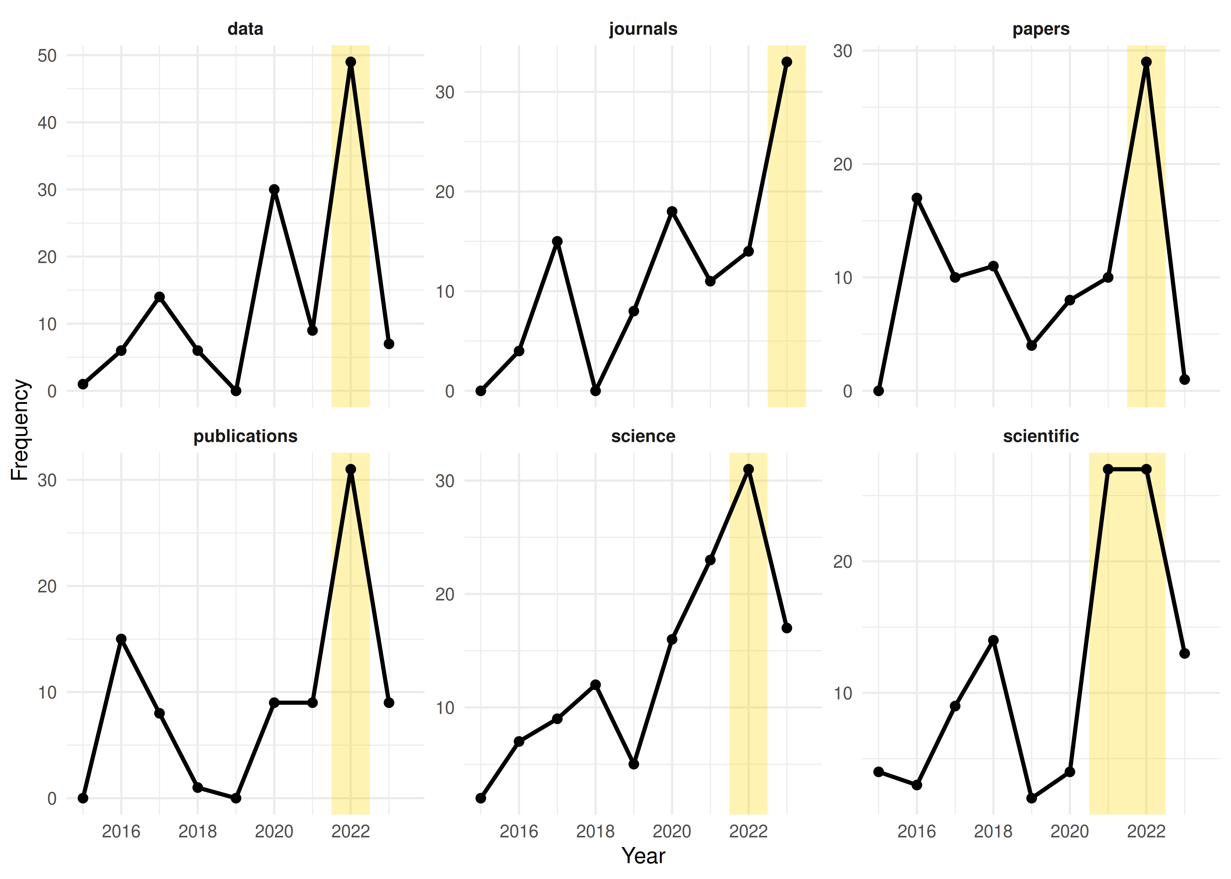
Figure 26.1: Temporal trajectories of emerging keywords with burst periods highlighted.
26.4.5 Rolling-window topic tracking
window_size <- 3
years <- sort(unique(text_df$year))
windows <- years[1:(length(years) - window_size + 1)]

window_top_terms <- map_dfr(windows, function(start_year) {
  end_year <- start_year + window_size - 1
  docs <- docvars(dfmat, "year") >= start_year &
          docvars(dfmat, "year") <= end_year
  if (sum(docs) < 10) return(tibble())
  top <- topfeatures(dfmat[docs, ], 10)
  tibble(window = glue("{start_year}-{end_year}"),
         term = names(top), frequency = unname(top))
})
window_top_terms |>
  group_by(window) |>
  slice_max(frequency, n = 8) |>
  mutate(term = reorder_within(term, frequency, window)) |>
  ggplot(aes(x = frequency, y = term)) +
  geom_col(fill = palette_sci(1)) +
  facet_wrap(~ window, scales = "free_y", ncol = 3) +
  scale_y_reordered() +
  labs(x = "Frequency", y = NULL) +
  theme_sci(base_size = 8)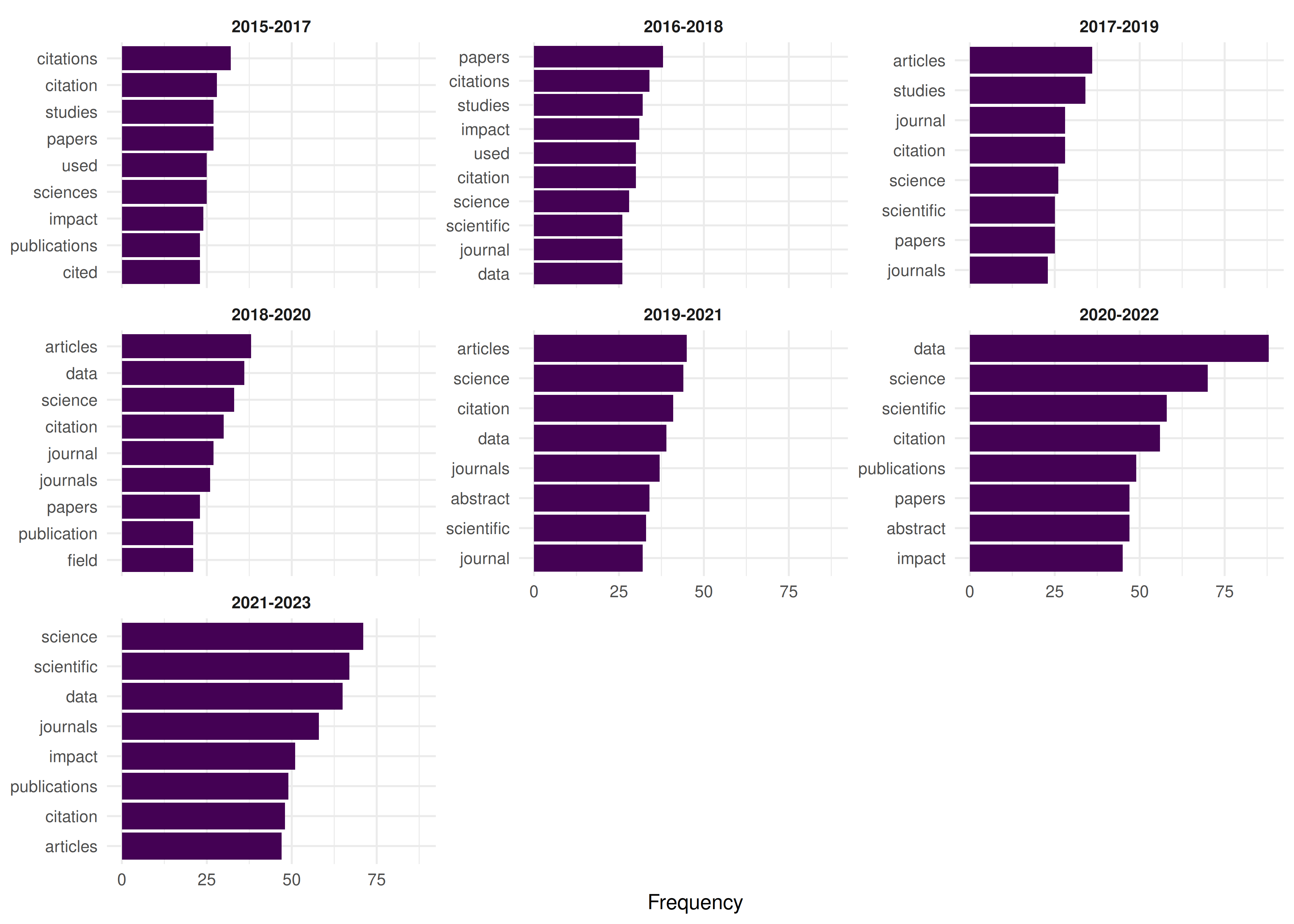
Figure 26.2: Top terms in each 3-year rolling window, showing vocabulary evolution.
26.5 Diagnostics and interpretation
- Baseline effects: A keyword going from 2 to 6 occurrences shows 200% growth but may not represent meaningful emergence. Set minimum frequency thresholds before computing growth rates.
- Database artefacts: A newly indexed journal or a batch import of conference proceedings can create spurious “bursts”. Cross-check with independent evidence.
- Burst duration: Short bursts (1 year) may reflect a single influential paper or a special issue. Sustained bursts (3+ years) more likely indicate genuine emergence.
- Window sensitivity: Rolling-window results change with window width. Report the chosen width and test sensitivity with wider and narrower windows.
26.7 Limitations and responsible use
- Emergence is retrospective. By the time bibliometric methods detect emergence, the topic has already gained momentum. These methods identify “recently emerged” topics, not future breakthroughs.
- Coverage bias. OpenAlex coverage has expanded rapidly, meaning recent years have more records. Growth rates may reflect database growth rather than intellectual emergence (Priem et al. 2022).
- Language of emergence. English-language terms dominate; emerging topics in non-English literatures may be invisible until translated or adopted by English-language publications.
- Not predictive. Burst detection identifies past patterns. It does not predict which topics will continue growing. Many bursts are transient (Kleinberg 2003).
- Strategic gaming. If emergence metrics are used for funding decisions, researchers may strategically choose “hot” keywords, creating feedback loops (Hicks et al. 2015).
26.9 Common pitfalls
- Confusing absolute growth with relative emergence. A field that publishes 10,000 papers/year growing by 5% adds 500 papers. A niche area growing from 10 to 30 papers shows 200% growth. The niche area is “emerging” but the large field is adding more absolute volume.
- Not controlling for corpus growth. If the overall number of publications in the corpus grows, all keywords will grow. Use relative frequency (keyword count / total documents) rather than absolute counts.
- Overreacting to single-year spikes. One conference proceedings volume or special issue can create a one-year spike. Require multi-year sustained growth before declaring emergence.
- Ignoring synonyms. “Deep learning” and “neural networks” may both refer to the same emerging trend. Merge synonyms before analysis.
26.10 Exercises
Relative burst detection. Modify the burst detection to use relative frequency (keyword proportion) instead of absolute counts. Do the same terms still burst?
Emergence by journal. Compare the most frequent emerging keywords in two different journals. Do they share emerging topics or focus on different frontiers?
Novelty scoring. For each document, compute its cosine distance to the centroid of all prior-year documents (using TF-IDF vectors). Plot novelty scores over time. Are recent papers becoming more or less novel?
Validation. Select 5 terms identified as “emerging” by burst detection. Search for qualitative evidence (review articles, conference themes) confirming their emergence. What is the false positive rate?
26.11 Solutions
Solutions are provided in 2.11.
26.12 Further reading
- Kleinberg (2003) — Bursty patterns in temporal data: the foundational burst detection algorithm.
- Solla Price (1963) — Early observations on the growth of scientific literature and research fronts.
- Priem et al. (2022) — OpenAlex temporal coverage patterns relevant to emergence detection.
- Callon et al. (1983) — Co-word dynamics; an early approach to tracking topical evolution.
26.13 Session info
#> R version 4.4.1 (2024-06-14)
#> Platform: x86_64-pc-linux-gnu
#> Running under: Ubuntu 24.04.4 LTS
#>
#> Matrix products: default
#> BLAS:   /usr/lib/x86_64-linux-gnu/openblas-pthread/libblas.so.3
#> LAPACK: /usr/lib/x86_64-linux-gnu/openblas-pthread/libopenblasp-r0.3.26.so;  LAPACK version 3.12.0
#>
#> locale:
#>  [1] LC_CTYPE=C.UTF-8       LC_NUMERIC=C           LC_TIME=C.UTF-8
#>  [4] LC_COLLATE=C.UTF-8     LC_MONETARY=C.UTF-8    LC_MESSAGES=C.UTF-8
#>  [7] LC_PAPER=C.UTF-8       LC_NAME=C              LC_ADDRESS=C
#> [10] LC_TELEPHONE=C         LC_MEASUREMENT=C.UTF-8 LC_IDENTIFICATION=C
#>
#> time zone: UTC
#> tzcode source: system (glibc)
#>
#> attached base packages:
#> [1] stats     graphics  grDevices utils     datasets  methods   base
#>
#> other attached packages:
#>  [1] uwot_0.2.4                Matrix_1.7-0
#>  [3] word2vec_0.4.1            stm_1.3.8
#>  [5] topicmodels_0.2-17        quanteda.textstats_0.97.2
#>  [7] visNetwork_2.1.4          ggraph_2.2.2
#>  [9] tidygraph_1.3.1           igraph_2.3.2
#> [11] quanteda_4.4              pdftools_3.9.0
#> [13] arrow_24.0.0              bibliometrix_5.4.0
#> [15] RefManageR_1.4.0          bib2df_1.1.2.0
#> [17] rcrossref_1.2.1           gt_1.3.0
#> [19] tidytext_0.4.3            glue_1.8.1
#> [21] openalexR_3.0.1           lubridate_1.9.5
#> [23] forcats_1.0.1             stringr_1.6.0
#> [25] dplyr_1.2.1               purrr_1.2.2
#> [27] readr_2.2.0               tidyr_1.3.2
#> [29] tibble_3.3.1              ggplot2_4.0.3
#> [31] tidyverse_2.0.0
#>
#> loaded via a namespace (and not attached):
#>   [1] bibtex_0.5.2           RColorBrewer_1.1-3     rstudioapi_0.18.0
#>   [4] jsonlite_2.0.0         magrittr_2.0.5         modeltools_0.2-24
#>   [7] farver_2.1.2           rmarkdown_2.31         fs_2.1.0
#>  [10] vctrs_0.7.3            memoise_2.0.1          askpass_1.2.1
#>  [13] base64enc_0.1-6        htmltools_0.5.9        contentanalysis_1.0.0
#>  [16] curl_7.1.0             janeaustenr_1.0.0      cellranger_1.1.0
#>  [19] sass_0.4.10            bslib_0.11.0           htmlwidgets_1.6.4
#>  [22] tokenizers_0.3.0       plyr_1.8.9             httr2_1.2.2
#>  [25] plotly_4.12.0          cachem_1.1.0           dimensionsR_0.0.3
#>  [28] mime_0.13              lifecycle_1.0.5        pkgconfig_2.0.3
#>  [31] R6_2.6.1               fastmap_1.2.0          shiny_1.13.0
#>  [34] digest_0.6.39          patchwork_1.3.2        shinycssloaders_1.1.0
#>  [37] rprojroot_2.1.1        RSpectra_0.16-2        SnowballC_0.7.1
#>  [40] labeling_0.4.3         urltools_1.7.3.1       timechange_0.4.0
#>  [43] polyclip_1.10-7        httr_1.4.8             compiler_4.4.1
#>  [46] here_1.0.2             bit64_4.8.0            withr_3.0.2
#>  [49] S7_0.2.2               backports_1.5.1        viridis_0.6.5
#>  [52] ggforce_0.5.0          MASS_7.3-60.2          rappdirs_0.3.4
#>  [55] bibliometrixData_0.3.0 tools_4.4.1            otel_0.2.0
#>  [58] stopwords_2.3          zip_2.3.3              httpuv_1.6.17
#>  [61] rentrez_1.2.4          promises_1.5.0         grid_4.4.1
#>  [64] stringdist_0.9.17      reshape2_1.4.5         generics_0.1.4
#>  [67] gtable_0.3.6           tzdb_0.5.0             rscopus_0.9.0
#>  [70] ca_0.71.1              data.table_1.18.4      hms_1.1.4
#>  [73] xml2_1.5.2             utf8_1.2.6             ggrepel_0.9.8
#>  [76] pillar_1.11.1          nsyllable_1.0.1        vroom_1.7.1
#>  [79] later_1.4.8            tweenr_2.0.3           brand.yml_0.1.0
#>  [82] lattice_0.22-6         FNN_1.1.4.1            bit_4.6.0
#>  [85] tidyselect_1.2.1       tm_0.7-18              miniUI_0.1.2
#>  [88] downlit_0.4.5          knitr_1.51             gridExtra_2.3
#>  [91] NLP_0.3-2              bookdown_0.46          stats4_4.4.1
#>  [94] crul_1.6.0             xfun_0.57              graphlayouts_1.2.3
#>  [97] matrixStats_1.5.0      DT_0.34.0              humaniformat_0.6.0
#> [100] stringi_1.8.7          lazyeval_0.2.3         qpdf_1.4.1
#> [103] yaml_2.3.12            evaluate_1.0.5         codetools_0.2-20
#> [106] httpcode_0.3.0         cli_3.6.6              xtable_1.8-8
#> [109] jquerylib_0.1.4        dichromat_2.0-0.1      Rcpp_1.1.1-1.1
#> [112] readxl_1.4.5           triebeard_0.4.1        XML_3.99-0.23
#> [115] parallel_4.4.1         assertthat_0.2.1       pubmedR_1.0.2
#> [118] slam_0.1-55            viridisLite_0.4.3      scales_1.4.0
#> [121] crayon_1.5.3           openxlsx_4.2.8.1       rlang_1.2.0
#> [124] fastmatch_1.1-8