22 Text Mining Bibliographic Corpora
22.1 Learning objectives
After completing this chapter, you will be able to:
- Build a text corpus from OpenAlex titles and abstracts
- Apply standard preprocessing steps: tokenisation, stopword removal, stemming
- Construct a document-term matrix (DTM) and a document-feature matrix (DFM)
- Compute TF-IDF weights to identify distinctive terms
- Visualise term frequency patterns across time or groups
22.3 Conceptual background
Bibliometric metadata — titles, abstracts, and keywords — constitutes a rich but noisy text corpus. Text mining transforms this unstructured data into structured representations suitable for statistical analysis. The pipeline typically follows three stages: preprocessing, representation, and analysis.
Preprocessing converts raw text into a standardised form. Tokenisation splits text into individual words or n-grams. Lowercasing removes case variation. Stopword removal eliminates high-frequency function words (“the”, “of”, “and”) that carry little topical information. Stemming or lemmatisation reduces words to their root forms (“computing”, “computed”, “computation” → “comput” or “compute”). Each step involves trade-offs: aggressive stemming can merge distinct concepts, while minimal preprocessing retains noise.
The document-term matrix (DTM) or document-feature matrix (DFM) is the fundamental representation. Rows are documents; columns are terms; cells contain counts or weights. Raw term frequencies overweight common words. TF-IDF (term frequency–inverse document frequency) addresses this by upweighting terms that are frequent in a document but rare across the corpus, highlighting words that distinguish one document from others.
quanteda (Aria and Cuccurullo 2017) provides a fast, well-designed toolkit for text analysis in R. Its corpus → tokens → dfm pipeline integrates naturally with the tidyverse. For very large corpora, quanteda uses sparse matrix representations that scale to millions of documents.
Text mining complements network-based methods (18.3). Co-word networks reveal term associations; text mining provides the frequency distributions, temporal trends, and discriminative features that characterise a field’s vocabulary.
22.4 Worked example
22.4.1 Building a text corpus
works <- oa_fetch(
  entity = "works",
  primary_location.source.id = "S148561398",
  from_publication_date = "2019-01-01",
  to_publication_date = "2023-12-31",
  options = list(sample = 500, seed = 42)
)

text_df <- works |>
  filter(!is.na(abstract), nchar(abstract) > 50) |>
  transmute(
    doc_id = id,
    text = paste(display_name, abstract, sep = ". "),
    year = year(publication_date)
  )

cat(glue("Documents with abstracts: {nrow(text_df)}\n"))
#> Documents with abstracts: 132
corp <- corpus(text_df, docid_field = "doc_id", text_field = "text")
docvars(corp, "year") <- text_df$year

cat(glue("Corpus size: {ndoc(corp)} documents\n"))
#> Corpus size: 132 documents#> Total tokens: 3376922.4.2 Tokenisation and preprocessing
toks <- tokens(corp,
               remove_punct = TRUE,
               remove_numbers = TRUE,
               remove_symbols = TRUE) |>
  tokens_tolower() |>
  tokens_remove(stopwords("en")) |>
  tokens_remove(c("also", "however", "using", "based", "study",
                   "paper", "results", "research", "analysis")) |>
  tokens_wordstem()

cat(glue("Tokens after preprocessing: {sum(ntoken(toks))}\n"))
#> Tokens after preprocessing: 1692722.4.3 Document-feature matrix
dfmat <- dfm(toks) |>
  dfm_trim(min_termfreq = 5, min_docfreq = 3)

cat(glue("DFM dimensions: {nrow(dfmat)} docs x {ncol(dfmat)} features\n"))
#> DFM dimensions: 132 docs x 712 features#> Sparsity: 91%
top_terms <- topfeatures(dfmat, 20) |>
  enframe(name = "term", value = "frequency") |>
  mutate(term = fct_reorder(term, frequency))

ggplot(top_terms, aes(x = frequency, y = term)) +
  geom_col(fill = palette_sci(1)) +
  labs(x = "Frequency", y = NULL) +
  theme_sci()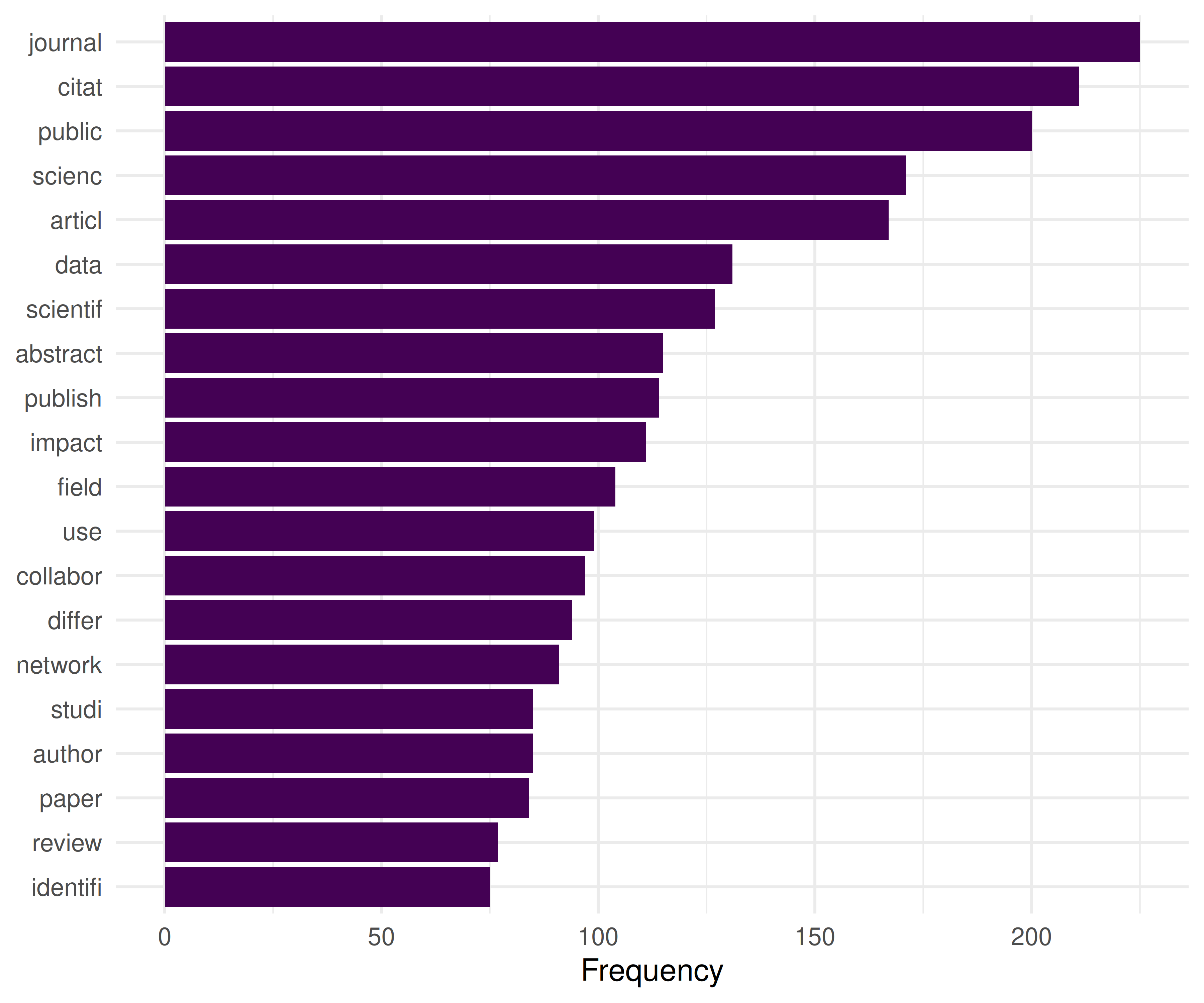
Figure 22.1: Top 20 most frequent terms in the Scientometrics corpus.
22.4.4 TF-IDF weighting
dfmat_tfidf <- dfm_tfidf(dfmat)

tfidf_by_year <- text_df |>
  group_by(year) |>
  group_keys() |>
  pull(year) |>
  map_dfr(function(yr) {
    docs <- docvars(dfmat_tfidf, "year") == yr
    if (sum(docs) < 5) return(tibble())
    top <- topfeatures(dfmat_tfidf[docs, ], 10)
    tibble(year = yr, term = names(top), tfidf = unname(top))
  })

tfidf_by_year |>
  group_by(year) |>
  slice_max(tfidf, n = 5) |>
  gt() |>
fmt_number(columns = tfidf, decimals = 1)| term | tfidf |
|---|---|
| 2019 | |
| citat | 17.2 |
| usag | 16.7 |
| peer | 14.8 |
| econom | 13.4 |
| review | 12.3 |
| 2020 | |
| lis | 30.4 |
| clinic | 18.8 |
| topic | 18.2 |
| practic | 18.2 |
| articl | 17.8 |
| 2021 | |
| predatori | 32.9 |
| retract | 27.3 |
| journal | 26.9 |
| covid-19 | 25.9 |
| oa | 25.8 |
| 2022 | |
| citat | 28.8 |
| univers | 25.4 |
| network | 24.4 |
| academ | 21.1 |
| perform | 20.9 |
| 2023 | |
| collabor | 20.5 |
| author | 20.0 |
| guidelin | 19.7 |
| femal | 19.5 |
| countri | 19.3 |
22.4.5 Term frequency over time
target_terms <- c("bibliometr", "open", "network", "impact", "collabor")

freq_by_year <- map_dfr(unique(text_df$year), function(yr) {
  docs <- docvars(dfmat, "year") == yr
  if (sum(docs) < 5) return(tibble())
  freq <- colSums(dfmat[docs, ]) / sum(dfmat[docs, ])
  tibble(
    year = yr,
    term = target_terms,
    rel_freq = freq[target_terms]
  )
})

ggplot(freq_by_year, aes(x = year, y = rel_freq, colour = term)) +
  geom_line(linewidth = 1) +
  geom_point(size = 2) +
  scale_colour_manual(values = palette_sci(length(target_terms))) +
  scale_y_continuous(labels = scales::percent_format(accuracy = 0.01)) +
  labs(x = "Year", y = "Relative frequency", colour = "Term") +
  theme_sci()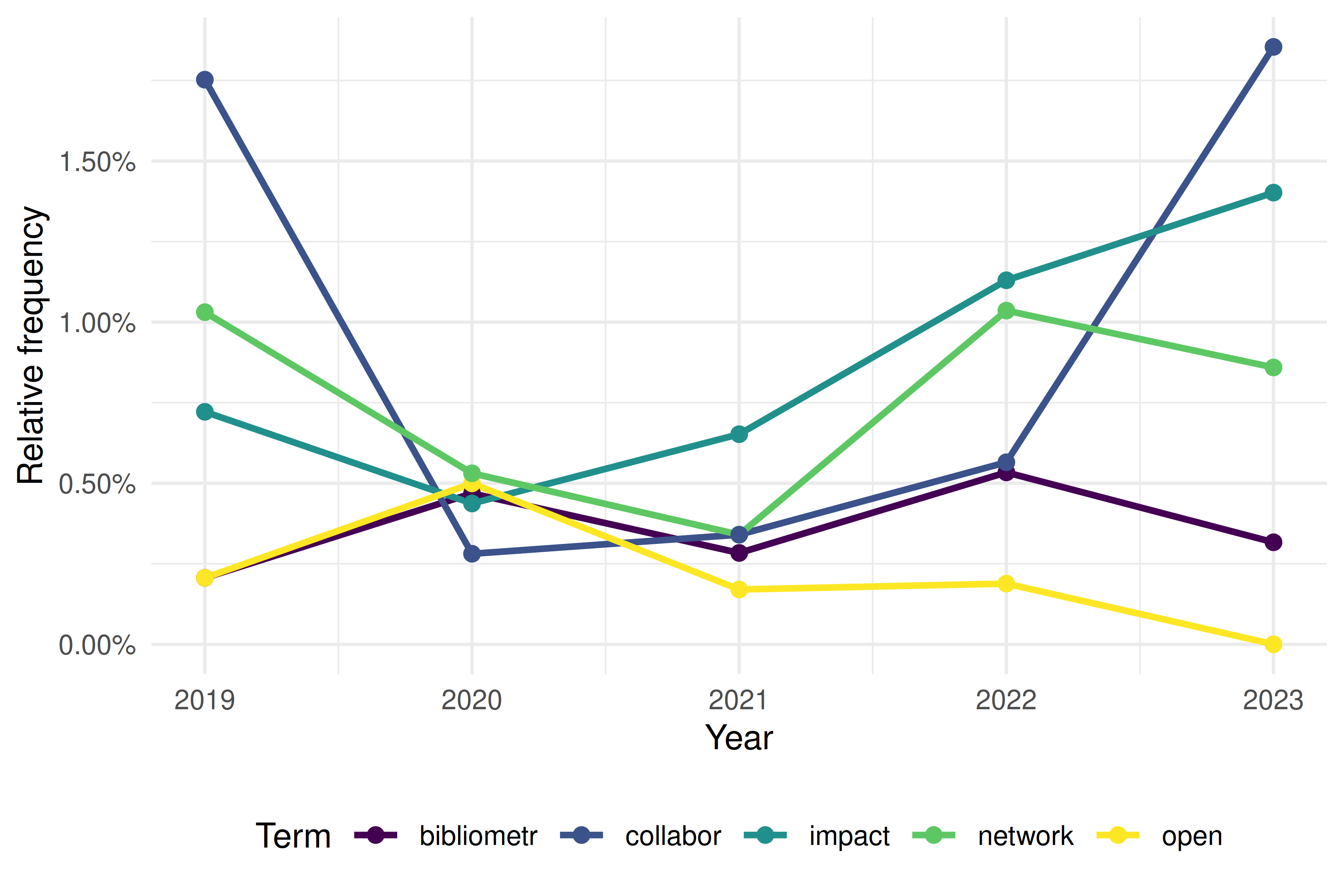
Figure 22.2: Relative frequency of selected terms over time.
22.5 Diagnostics and interpretation
- Vocabulary size vs. documents: A typical DFM has far more features than documents. Trim aggressively (minimum document frequency of 3–5) to reduce noise and computation.
- Sparsity: Bibliometric DFMs are typically 95–99% sparse. This is normal. Sparse matrix representations keep memory usage manageable.
- Preprocessing sensitivity: Results change with preprocessing choices. Always report stopword list, stemming method, and trimming thresholds.
- Abstract availability: Not all OpenAlex records have abstracts. Report the coverage rate and consider whether missing abstracts introduce bias (e.g., older papers, certain publishers).
22.7 Limitations and responsible use
- Abstracts are summaries. They capture the main claims but miss nuance, methodology details, and negative results. Full-text analysis (9.3) provides richer data but is harder to obtain.
- Language bias. Text mining tools work best for English. Non-English abstracts may be poorly tokenised, incorrectly stemmed, or excluded entirely. This biases results toward Anglophone research (Visser et al. 2021).
- Stemming conflates concepts. “Stem” and “stemming” are merged, but so are “cell” (biology) and “cell” (spreadsheet). Lemmatisation is more precise but slower.
- Bag-of-words ignores context. TF-IDF and frequency-based methods treat documents as unordered collections of words. Phrase meaning (“machine learning” vs. “learning machine”) is lost unless you use n-grams or embeddings (25.3).
22.9 Common pitfalls
- Not removing domain-specific stop words. Generic stopword lists miss terms like “study”, “results”, “paper” that dominate academic text without conveying topical information.
- Applying TF-IDF before trimming. Rare terms get extreme TF-IDF scores. Trim the DFM first, then apply TF-IDF.
- Comparing raw frequencies across groups of different sizes. A year with 200 papers will have higher raw counts than a year with 50. Always normalise to relative frequency.
- Stemming titles but not abstracts (or vice versa). Apply identical preprocessing to all text fields.
22.10 Exercises
Bigram analysis. Build a DFM using bigrams (two-word sequences) instead of unigrams. What meaningful phrases emerge that single words miss?
Lexical diversity. Compute the type-token ratio (TTR) for each publication year. Is the vocabulary growing more diverse or more standardised over time?
Keyness analysis. Use
quanteda.textstats::textstat_keyness()to identify terms that distinguish one year from all others. What terms characterise 2023 specifically?Preprocessing sensitivity. Run the same analysis with and without stemming. How do the top terms differ? Which version is more interpretable?
22.11 Solutions
Solutions are provided in 2.11.
22.13 Session info
#> R version 4.4.1 (2024-06-14)
#> Platform: x86_64-pc-linux-gnu
#> Running under: Ubuntu 24.04.4 LTS
#>
#> Matrix products: default
#> BLAS:   /usr/lib/x86_64-linux-gnu/openblas-pthread/libblas.so.3
#> LAPACK: /usr/lib/x86_64-linux-gnu/openblas-pthread/libopenblasp-r0.3.26.so;  LAPACK version 3.12.0
#>
#> locale:
#>  [1] LC_CTYPE=C.UTF-8       LC_NUMERIC=C           LC_TIME=C.UTF-8
#>  [4] LC_COLLATE=C.UTF-8     LC_MONETARY=C.UTF-8    LC_MESSAGES=C.UTF-8
#>  [7] LC_PAPER=C.UTF-8       LC_NAME=C              LC_ADDRESS=C
#> [10] LC_TELEPHONE=C         LC_MEASUREMENT=C.UTF-8 LC_IDENTIFICATION=C
#>
#> time zone: UTC
#> tzcode source: system (glibc)
#>
#> attached base packages:
#> [1] stats     graphics  grDevices utils     datasets  methods   base
#>
#> other attached packages:
#>  [1] quanteda.textstats_0.97.2 visNetwork_2.1.4
#>  [3] ggraph_2.2.2              tidygraph_1.3.1
#>  [5] igraph_2.3.2              quanteda_4.4
#>  [7] pdftools_3.9.0            arrow_24.0.0
#>  [9] bibliometrix_5.4.0        RefManageR_1.4.0
#> [11] bib2df_1.1.2.0            rcrossref_1.2.1
#> [13] gt_1.3.0                  tidytext_0.4.3
#> [15] glue_1.8.1                openalexR_3.0.1
#> [17] lubridate_1.9.5           forcats_1.0.1
#> [19] stringr_1.6.0             dplyr_1.2.1
#> [21] purrr_1.2.2               readr_2.2.0
#> [23] tidyr_1.3.2               tibble_3.3.1
#> [25] ggplot2_4.0.3             tidyverse_2.0.0
#>
#> loaded via a namespace (and not attached):
#>   [1] bibtex_0.5.2           RColorBrewer_1.1-3     rstudioapi_0.18.0
#>   [4] jsonlite_2.0.0         magrittr_2.0.5         farver_2.1.2
#>   [7] rmarkdown_2.31         fs_2.1.0               vctrs_0.7.3
#>  [10] memoise_2.0.1          askpass_1.2.1          base64enc_0.1-6
#>  [13] htmltools_0.5.9        contentanalysis_1.0.0  curl_7.1.0
#>  [16] janeaustenr_1.0.0      cellranger_1.1.0       sass_0.4.10
#>  [19] bslib_0.11.0           htmlwidgets_1.6.4      tokenizers_0.3.0
#>  [22] plyr_1.8.9             httr2_1.2.2            plotly_4.12.0
#>  [25] cachem_1.1.0           dimensionsR_0.0.3      mime_0.13
#>  [28] lifecycle_1.0.5        pkgconfig_2.0.3        Matrix_1.7-0
#>  [31] R6_2.6.1               fastmap_1.2.0          shiny_1.13.0
#>  [34] digest_0.6.39          patchwork_1.3.2        shinycssloaders_1.1.0
#>  [37] rprojroot_2.1.1        SnowballC_0.7.1        labeling_0.4.3
#>  [40] urltools_1.7.3.1       timechange_0.4.0       polyclip_1.10-7
#>  [43] httr_1.4.8             compiler_4.4.1         here_1.0.2
#>  [46] bit64_4.8.0            withr_3.0.2            S7_0.2.2
#>  [49] backports_1.5.1        viridis_0.6.5          ggforce_0.5.0
#>  [52] MASS_7.3-60.2          rappdirs_0.3.4         bibliometrixData_0.3.0
#>  [55] tools_4.4.1            otel_0.2.0             stopwords_2.3
#>  [58] zip_2.3.3              httpuv_1.6.17          rentrez_1.2.4
#>  [61] promises_1.5.0         grid_4.4.1             stringdist_0.9.17
#>  [64] generics_0.1.4         gtable_0.3.6           tzdb_0.5.0
#>  [67] rscopus_0.9.0          ca_0.71.1              data.table_1.18.4
#>  [70] hms_1.1.4              xml2_1.5.2             utf8_1.2.6
#>  [73] ggrepel_0.9.8          pillar_1.11.1          nsyllable_1.0.1
#>  [76] vroom_1.7.1            later_1.4.8            tweenr_2.0.3
#>  [79] brand.yml_0.1.0        lattice_0.22-6         bit_4.6.0
#>  [82] tidyselect_1.2.1       miniUI_0.1.2           downlit_0.4.5
#>  [85] knitr_1.51             gridExtra_2.3          bookdown_0.46
#>  [88] crul_1.6.0             xfun_0.57              graphlayouts_1.2.3
#>  [91] DT_0.34.0              humaniformat_0.6.0     stringi_1.8.7
#>  [94] lazyeval_0.2.3         qpdf_1.4.1             yaml_2.3.12
#>  [97] evaluate_1.0.5         codetools_0.2-20       httpcode_0.3.0
#> [100] cli_3.6.6              xtable_1.8-8           jquerylib_0.1.4
#> [103] dichromat_2.0-0.1      Rcpp_1.1.1-1.1         readxl_1.4.5
#> [106] triebeard_0.4.1        XML_3.99-0.23          parallel_4.4.1
#> [109] assertthat_0.2.1       pubmedR_1.0.2          viridisLite_0.4.3
#> [112] scales_1.4.0           crayon_1.5.3           openxlsx_4.2.8.1
#> [115] rlang_1.2.0            fastmatch_1.1-8