25 Embeddings for Scientometrics
25.1 Learning objectives
After completing this chapter, you will be able to:
- Explain how word and document embeddings differ from bag-of-words representations
- Train simple word embeddings on a bibliometric corpus
- Use pre-trained embeddings to compute document similarity
- Apply UMAP or t-SNE to visualise document clusters in embedding space
- Assess when embeddings add value over simpler text representations
25.3 Conceptual background
Bag-of-words representations (22.3) treat each word as an independent dimension. “Citation analysis” and “bibliometric study” share no features despite being semantically related. Word embeddings address this by mapping words into a dense, low-dimensional vector space where semantically similar words are close together. The word2vec algorithm learns these representations by predicting words from their context (skip-gram) or context from words (CBOW) in a large training corpus.
Document embeddings extend the idea to whole documents. Simple approaches average the word vectors of a document’s words (mean pooling). More sophisticated approaches include Doc2Vec (Paragraph Vector), which learns document-specific vectors alongside word vectors, and transformer-based models like SPECTER, which is pre-trained on scientific paper titles and abstracts using citation-based training signals.
For scientometrics, embeddings enable several applications:
- Semantic similarity: Finding papers with similar meaning, even when they use different terminology.
- Clustering: Grouping papers by content in embedding space, complementing topic models (23.3).
- Visualisation: Projecting embeddings to 2D with UMAP or t-SNE to create interpretable “maps” of a corpus.
- Anomaly detection: Identifying papers that are semantically distant from their assigned field or cluster.
The trade-off is interpretability: while TF-IDF features are directly readable (the word “citation” has a specific weight), embedding dimensions are opaque. Embeddings are powerful for similarity and clustering but resist the kind of term-level interpretation that co-word analysis provides.
25.4 Worked example
25.4.1 Preparing text data
works <- oa_fetch(
  entity = "works",
  primary_location.source.id = "S148561398",
  from_publication_date = "2019-01-01",
  to_publication_date = "2023-12-31",
  options = list(sample = 400, seed = 42)
)

text_df <- works |>
  filter(!is.na(abstract), nchar(abstract) > 100) |>
  transmute(
    doc_id = id,
    title = display_name,
    text = paste(display_name, abstract, sep = ". "),
    year = year(publication_date),
    cited_by_count
  )

cat(glue("Documents for embedding: {nrow(text_df)}\n"))
#> Documents for embedding: 10225.4.2 Training word2vec embeddings
clean_text <- text_df$text |>
  str_to_lower() |>
  str_replace_all("[^a-z ]", " ") |>
  str_squish()

model <- word2vec(clean_text, dim = 100, iter = 20, min_count = 3,
                  type = "skip-gram", threads = 1)

cat(glue("Vocabulary size: {nrow(as.matrix(model))}\n"))
#> Vocabulary size: 1330
if ("citation" %in% rownames(as.matrix(model))) {
  nn <- predict(model, newdata = "citation", type = "nearest", top_n = 10)
  cat("Nearest neighbours of 'citation':\n")
  print(nn)
}
#> Nearest neighbours of 'citation':
#> $citation
#> term1 term2 similarity rank
#> 1 citation meanings 0.774 1
#> 2 citation percentile 0.762 2
#> 3 citation normalised 0.761 3
#> 4 citation sentiment 0.747 4
#> 5 citation score 0.742 5
#> 6 citation citations 0.734 6
#> 7 citation mean 0.733 7
#> 8 citation function 0.722 8
#> 9 citation belong 0.721 9
#> 10 citation facilitate 0.716 1025.4.3 Computing document embeddings via mean pooling
word_matrix <- as.matrix(model)

doc_embed <- function(text, wm) {
  words <- str_split(str_to_lower(str_replace_all(text, "[^a-z ]", " ")),
                     "\\s+")[[1]]
  matched <- words[words %in% rownames(wm)]
  if (length(matched) == 0) return(rep(NA_real_, ncol(wm)))
  colMeans(wm[matched, , drop = FALSE])
}

doc_embeddings <- map(text_df$text, \(t) doc_embed(t, word_matrix))
embed_mat <- do.call(rbind, doc_embeddings)

valid <- complete.cases(embed_mat)
embed_mat <- embed_mat[valid, ]
text_df_valid <- text_df[valid, ]

cat(glue("Valid document embeddings: {nrow(embed_mat)}\n"))
#> Valid document embeddings: 10225.4.4 Dimensionality reduction with UMAP
umap_result <- umap(embed_mat, n_neighbors = 15, min_dist = 0.1,
                    n_components = 2, ret_model = FALSE)

text_df_valid$umap_x <- umap_result[, 1]
text_df_valid$umap_y <- umap_result[, 2]
ggplot(text_df_valid, aes(x = umap_x, y = umap_y, colour = factor(year))) +
  geom_point(alpha = 0.6, size = 1.5) +
  scale_colour_manual(values = palette_sci(n_distinct(text_df_valid$year))) +
  labs(x = "UMAP 1", y = "UMAP 2", colour = "Year") +
  theme_sci() +
  theme(axis.text = element_blank(), axis.ticks = element_blank())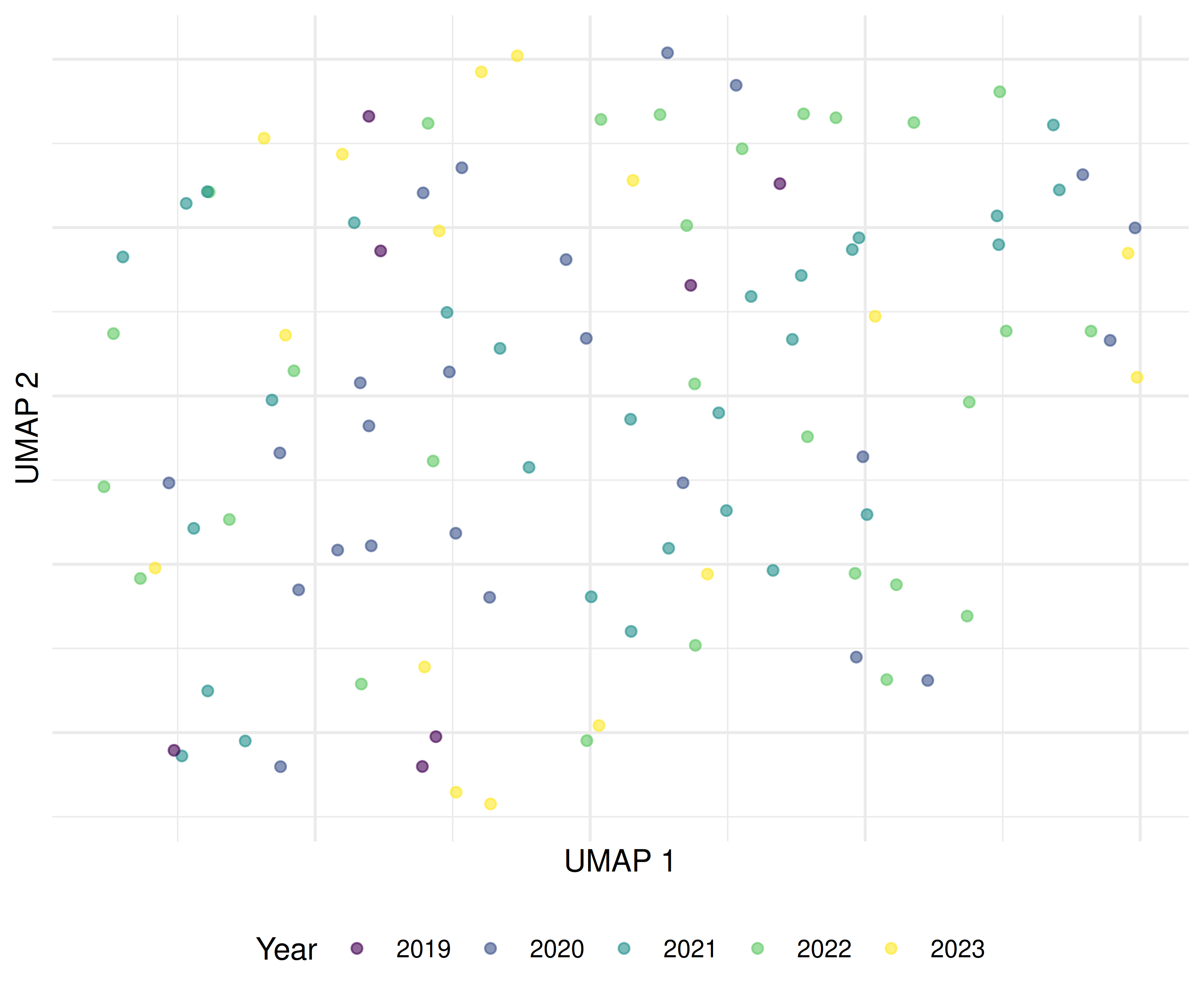
Figure 25.1: UMAP projection of document embeddings, coloured by publication year.
25.4.5 Document similarity search
cosine_sim <- function(a, b) sum(a * b) / (sqrt(sum(a^2)) * sqrt(sum(b^2)))

query_idx <- 1
sims <- map_dbl(seq_len(nrow(embed_mat)),
                \(i) cosine_sim(embed_mat[query_idx, ], embed_mat[i, ]))

top_similar <- order(sims, decreasing = TRUE)[2:6]

cat(glue("Query: {text_df_valid$title[query_idx]}\n\n"))
#> Query: How academic opinion leaders shape scientific ideas: an acknowledgment analysis
cat("Most similar documents:\n")#> Most similar documents:#> [0.926] Draw me Science[0.926] COVID-19 and the scientific publishing system: growth, open access and scientific fields[0.921] The state of social science research on COVID-19[0.915] How scientific research reacts to international public health emergencies: a global analysis of response patterns[0.907] Presence and consequences of positive words in scientific abstracts25.4.6 Embedding clusters vs. citation impact
ggplot(text_df_valid, aes(x = umap_x, y = umap_y,
                          colour = log1p(cited_by_count))) +
  geom_point(alpha = 0.6, size = 1.5) +
  scale_colour_viridis_c(option = "C", name = "log(cites + 1)") +
  labs(x = "UMAP 1", y = "UMAP 2") +
  theme_sci() +
  theme(axis.text = element_blank(), axis.ticks = element_blank())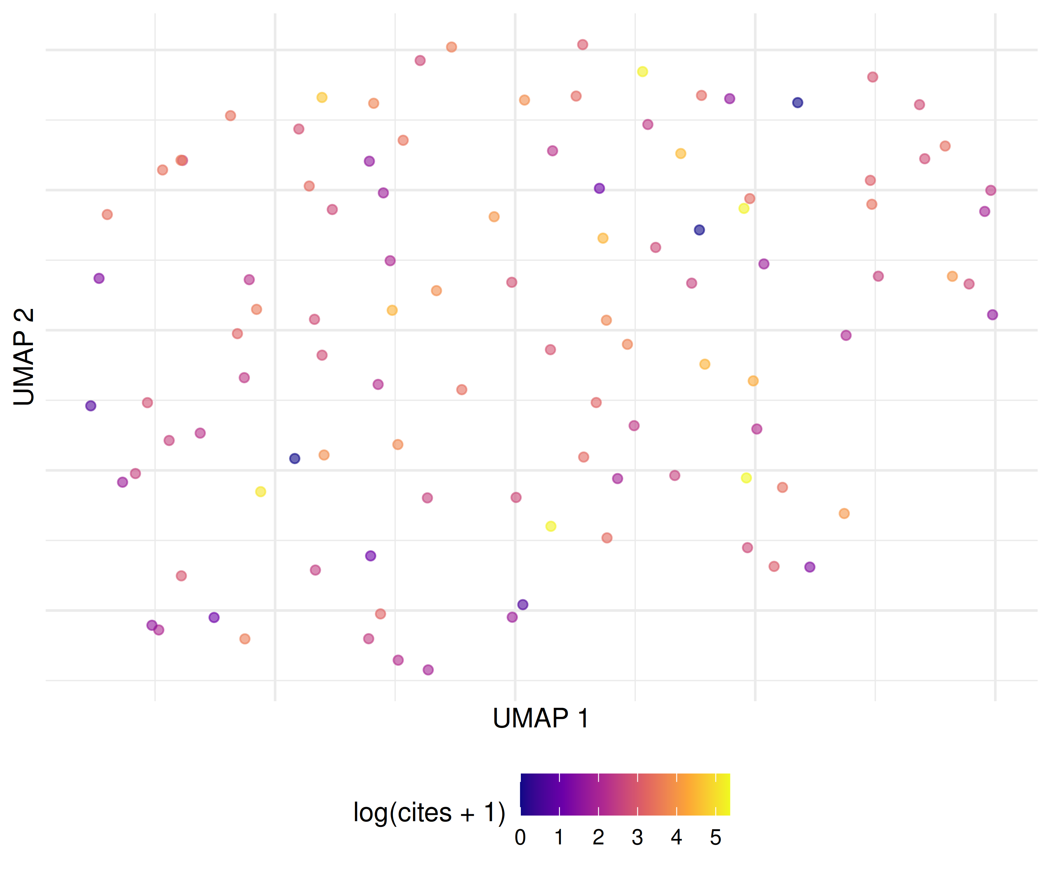
Figure 25.2: UMAP embedding coloured by citation impact (log scale).
25.5 Diagnostics and interpretation
- Vocabulary coverage: Check what fraction of abstract words appear in the embedding vocabulary. Low coverage (< 80%) indicates the training corpus is too small or preprocessing is too aggressive.
- Nearest neighbours: Inspect the nearest neighbours of key domain terms. If “citation” is closest to “references” and “bibliometric”, the embeddings capture domain structure.
- UMAP stability: UMAP is stochastic. Run with multiple seeds and check whether the global cluster structure is stable. Individual point positions will vary but clusters should persist.
- Embedding dimensionality: 100–300 dimensions is standard. Below 50, embeddings lose semantic resolution; above 300, training becomes slow with diminishing returns.
25.7 Limitations and responsible use
- Embeddings are opaque. Unlike TF-IDF weights, embedding dimensions have no interpretable meaning. You can measure similarity but not explain why two documents are similar without additional analysis.
- Training data bias. Embeddings reflect the biases of their training corpus. If the corpus overrepresents certain topics or perspectives, the embeddings will too.
- Small corpora produce poor embeddings. Word2vec needs tens of thousands of documents for reliable training. For small bibliometric corpora (< 1,000 papers), use pre-trained embeddings instead.
- UMAP/t-SNE distort distances. These methods preserve local structure but distort global distances. Documents that appear close in 2D may not be the most similar in high-dimensional space (Hicks et al. 2015).
25.9 Common pitfalls
- Training on too few documents. Word2vec on 200 abstracts produces unreliable embeddings. Use at least 5,000 documents or switch to pre-trained models.
- Averaging without weighting. Simple mean pooling treats every word equally. TF-IDF-weighted averaging gives more weight to distinctive terms and often produces better document embeddings.
- Over-interpreting UMAP clusters. Visual clusters in UMAP may reflect projection artifacts. Validate clusters with a separate method (e.g., k-means in the full embedding space).
- Comparing embeddings from different models. Embedding spaces are not aligned across different training runs. Cosine similarity is only meaningful within a single embedding space.
25.10 Exercises
Weighted averaging. Compute document embeddings using TF-IDF-weighted word vectors instead of simple means. Does the UMAP visualisation change?
K-means clustering. Apply k-means (k = 5, 8, 12) to the document embeddings. Compare the resulting clusters with LDA topics from 23.4. Do they agree?
Pre-trained embeddings. If available, use SPECTER embeddings (via reticulate and Python) instead of corpus-trained word2vec. How does similarity search quality change?
Analogy test. Test whether the word2vec model captures analogical relationships (e.g., “journal” - “article” + “book” ≈ “publisher”). What does the result tell you about the model?
25.11 Solutions
Solutions are provided in 2.11.
25.13 Session info
#> R version 4.4.1 (2024-06-14)
#> Platform: x86_64-pc-linux-gnu
#> Running under: Ubuntu 24.04.4 LTS
#>
#> Matrix products: default
#> BLAS:   /usr/lib/x86_64-linux-gnu/openblas-pthread/libblas.so.3
#> LAPACK: /usr/lib/x86_64-linux-gnu/openblas-pthread/libopenblasp-r0.3.26.so;  LAPACK version 3.12.0
#>
#> locale:
#>  [1] LC_CTYPE=C.UTF-8       LC_NUMERIC=C           LC_TIME=C.UTF-8
#>  [4] LC_COLLATE=C.UTF-8     LC_MONETARY=C.UTF-8    LC_MESSAGES=C.UTF-8
#>  [7] LC_PAPER=C.UTF-8       LC_NAME=C              LC_ADDRESS=C
#> [10] LC_TELEPHONE=C         LC_MEASUREMENT=C.UTF-8 LC_IDENTIFICATION=C
#>
#> time zone: UTC
#> tzcode source: system (glibc)
#>
#> attached base packages:
#> [1] stats     graphics  grDevices utils     datasets  methods   base
#>
#> other attached packages:
#>  [1] uwot_0.2.4                Matrix_1.7-0
#>  [3] word2vec_0.4.1            stm_1.3.8
#>  [5] topicmodels_0.2-17        quanteda.textstats_0.97.2
#>  [7] visNetwork_2.1.4          ggraph_2.2.2
#>  [9] tidygraph_1.3.1           igraph_2.3.2
#> [11] quanteda_4.4              pdftools_3.9.0
#> [13] arrow_24.0.0              bibliometrix_5.4.0
#> [15] RefManageR_1.4.0          bib2df_1.1.2.0
#> [17] rcrossref_1.2.1           gt_1.3.0
#> [19] tidytext_0.4.3            glue_1.8.1
#> [21] openalexR_3.0.1           lubridate_1.9.5
#> [23] forcats_1.0.1             stringr_1.6.0
#> [25] dplyr_1.2.1               purrr_1.2.2
#> [27] readr_2.2.0               tidyr_1.3.2
#> [29] tibble_3.3.1              ggplot2_4.0.3
#> [31] tidyverse_2.0.0
#>
#> loaded via a namespace (and not attached):
#>   [1] bibtex_0.5.2           RColorBrewer_1.1-3     rstudioapi_0.18.0
#>   [4] jsonlite_2.0.0         magrittr_2.0.5         modeltools_0.2-24
#>   [7] farver_2.1.2           rmarkdown_2.31         fs_2.1.0
#>  [10] vctrs_0.7.3            memoise_2.0.1          askpass_1.2.1
#>  [13] base64enc_0.1-6        htmltools_0.5.9        contentanalysis_1.0.0
#>  [16] curl_7.1.0             janeaustenr_1.0.0      cellranger_1.1.0
#>  [19] sass_0.4.10            bslib_0.11.0           htmlwidgets_1.6.4
#>  [22] tokenizers_0.3.0       plyr_1.8.9             httr2_1.2.2
#>  [25] plotly_4.12.0          cachem_1.1.0           dimensionsR_0.0.3
#>  [28] mime_0.13              lifecycle_1.0.5        pkgconfig_2.0.3
#>  [31] R6_2.6.1               fastmap_1.2.0          shiny_1.13.0
#>  [34] digest_0.6.39          patchwork_1.3.2        shinycssloaders_1.1.0
#>  [37] rprojroot_2.1.1        RSpectra_0.16-2        SnowballC_0.7.1
#>  [40] labeling_0.4.3         urltools_1.7.3.1       timechange_0.4.0
#>  [43] polyclip_1.10-7        httr_1.4.8             compiler_4.4.1
#>  [46] here_1.0.2             bit64_4.8.0            withr_3.0.2
#>  [49] S7_0.2.2               backports_1.5.1        viridis_0.6.5
#>  [52] ggforce_0.5.0          MASS_7.3-60.2          rappdirs_0.3.4
#>  [55] bibliometrixData_0.3.0 tools_4.4.1            otel_0.2.0
#>  [58] stopwords_2.3          zip_2.3.3              httpuv_1.6.17
#>  [61] rentrez_1.2.4          promises_1.5.0         grid_4.4.1
#>  [64] stringdist_0.9.17      reshape2_1.4.5         generics_0.1.4
#>  [67] gtable_0.3.6           tzdb_0.5.0             rscopus_0.9.0
#>  [70] ca_0.71.1              data.table_1.18.4      hms_1.1.4
#>  [73] xml2_1.5.2             utf8_1.2.6             ggrepel_0.9.8
#>  [76] pillar_1.11.1          nsyllable_1.0.1        vroom_1.7.1
#>  [79] later_1.4.8            tweenr_2.0.3           brand.yml_0.1.0
#>  [82] lattice_0.22-6         FNN_1.1.4.1            bit_4.6.0
#>  [85] tidyselect_1.2.1       tm_0.7-18              miniUI_0.1.2
#>  [88] downlit_0.4.5          knitr_1.51             gridExtra_2.3
#>  [91] NLP_0.3-2              bookdown_0.46          stats4_4.4.1
#>  [94] crul_1.6.0             xfun_0.57              graphlayouts_1.2.3
#>  [97] matrixStats_1.5.0      DT_0.34.0              humaniformat_0.6.0
#> [100] stringi_1.8.7          lazyeval_0.2.3         qpdf_1.4.1
#> [103] yaml_2.3.12            evaluate_1.0.5         codetools_0.2-20
#> [106] httpcode_0.3.0         cli_3.6.6              xtable_1.8-8
#> [109] jquerylib_0.1.4        dichromat_2.0-0.1      Rcpp_1.1.1-1.1
#> [112] readxl_1.4.5           triebeard_0.4.1        XML_3.99-0.23
#> [115] parallel_4.4.1         assertthat_0.2.1       pubmedR_1.0.2
#> [118] slam_0.1-55            viridisLite_0.4.3      scales_1.4.0
#> [121] crayon_1.5.3           openxlsx_4.2.8.1       rlang_1.2.0
#> [124] fastmatch_1.1-8