43 Case Study 5: Detecting Emerging Topics

43.1 Objective

Identify emerging topics in scientometrics research (2015–2023) using keyword burst detection and topic modelling, and validate findings against known developments in the field.

43.2 Setup

library(tidyverse)
library(openalexR)
library(quanteda)
library(quanteda.textstats)
library(topicmodels)
library(tidytext)
library(glue)
library(gt)

set.seed(20260509)

source(here::here("R", "api_helpers.R"))
source(here::here("R", "utils.R"))
source(here::here("R", "sci_palette.R"))

43.3 Data acquisition

works <- oa_fetch(
  entity = "works",
  primary_location.source.id = "S148561398",
  from_publication_date = "2015-01-01",
  to_publication_date = "2023-12-31",
  type = "article",
  options = list(sample = 600, seed = 42)
)

text_df <- works |>
  filter(!is.na(abstract), nchar(abstract) > 50) |>
  transmute(
    doc_id = id,
    text = paste(display_name, abstract, sep = ". "),
    year = year(publication_date)
  )

cat(glue("Documents: {nrow(text_df)}\n"))

#> Documents: 118

43.4 Keyword burst detection

corp <- corpus(text_df, docid_field = "doc_id", text_field = "text")
docvars(corp, "year") <- text_df$year

toks <- tokens(corp, remove_punct = TRUE, remove_numbers = TRUE) |>
  tokens_tolower() |>
  tokens_remove(stopwords("en")) |>
  tokens_remove(c("study", "paper", "results", "research", "analysis",
                   "also", "however", "using", "based"))

dfmat <- dfm(toks) |> dfm_trim(min_termfreq = 10, min_docfreq = 5)

kw_by_year <- quanteda::convert(dfm_group(dfmat, groups = year), to = "data.frame") |>
  pivot_longer(-doc_id, names_to = "term", values_to = "count") |>
  rename(year = doc_id) |>
  mutate(year = as.integer(year))

growth <- kw_by_year |>
  group_by(term) |>
  filter(sum(count) >= 20) |>
  arrange(year) |>
  mutate(growth = (count - lag(count)) / pmax(lag(count), 1)) |>
  ungroup() |>
  filter(!is.na(growth))

recent_growth <- growth |>
  filter(year >= 2021) |>
  group_by(term) |>
  summarise(mean_growth = mean(growth), total = sum(count), .groups = "drop") |>
  filter(mean_growth > 0) |>
  arrange(desc(mean_growth))

recent_growth |>
  head(15) |>
  mutate(term = fct_reorder(term, mean_growth)) |>
  ggplot(aes(x = mean_growth, y = term)) +
  geom_col(fill = palette_sci(1)) +
  scale_x_continuous(labels = scales::percent) +
  labs(x = "Mean growth rate (2021–2023)", y = NULL) +
  theme_sci()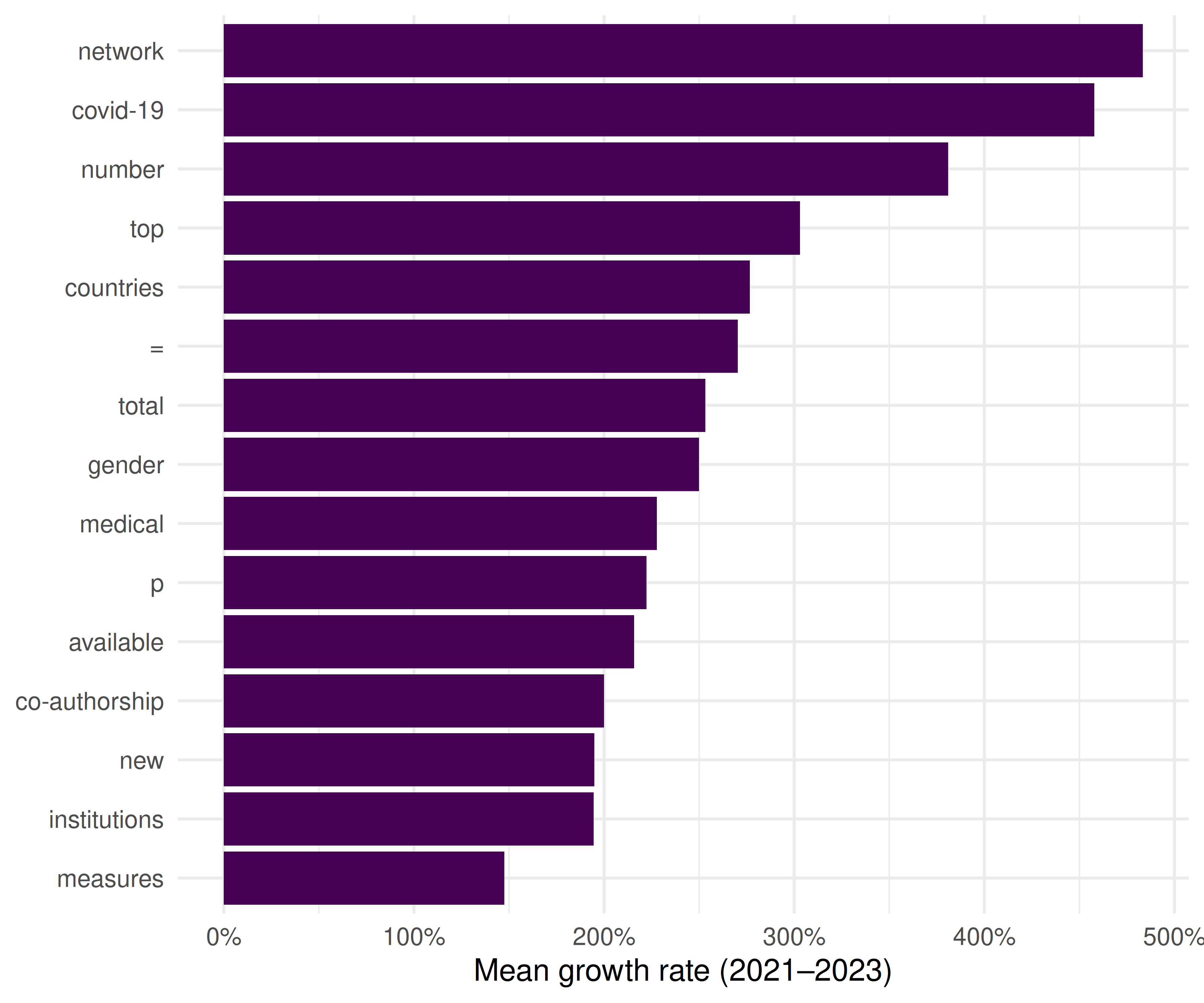

Figure 43.1: Top 15 fastest-growing keywords (2021–2023).

43.5 Keyword trajectories

emerging_terms <- recent_growth |> head(6) |> pull(term)

kw_by_year |>
  filter(term %in% emerging_terms) |>
  ggplot(aes(x = year, y = count, colour = term)) +
  geom_line(linewidth = 0.8) +
  geom_point(size = 1.5) +
  scale_colour_manual(values = palette_sci(length(emerging_terms))) +
  labs(x = "Year", y = "Frequency", colour = "Keyword") +
  theme_sci()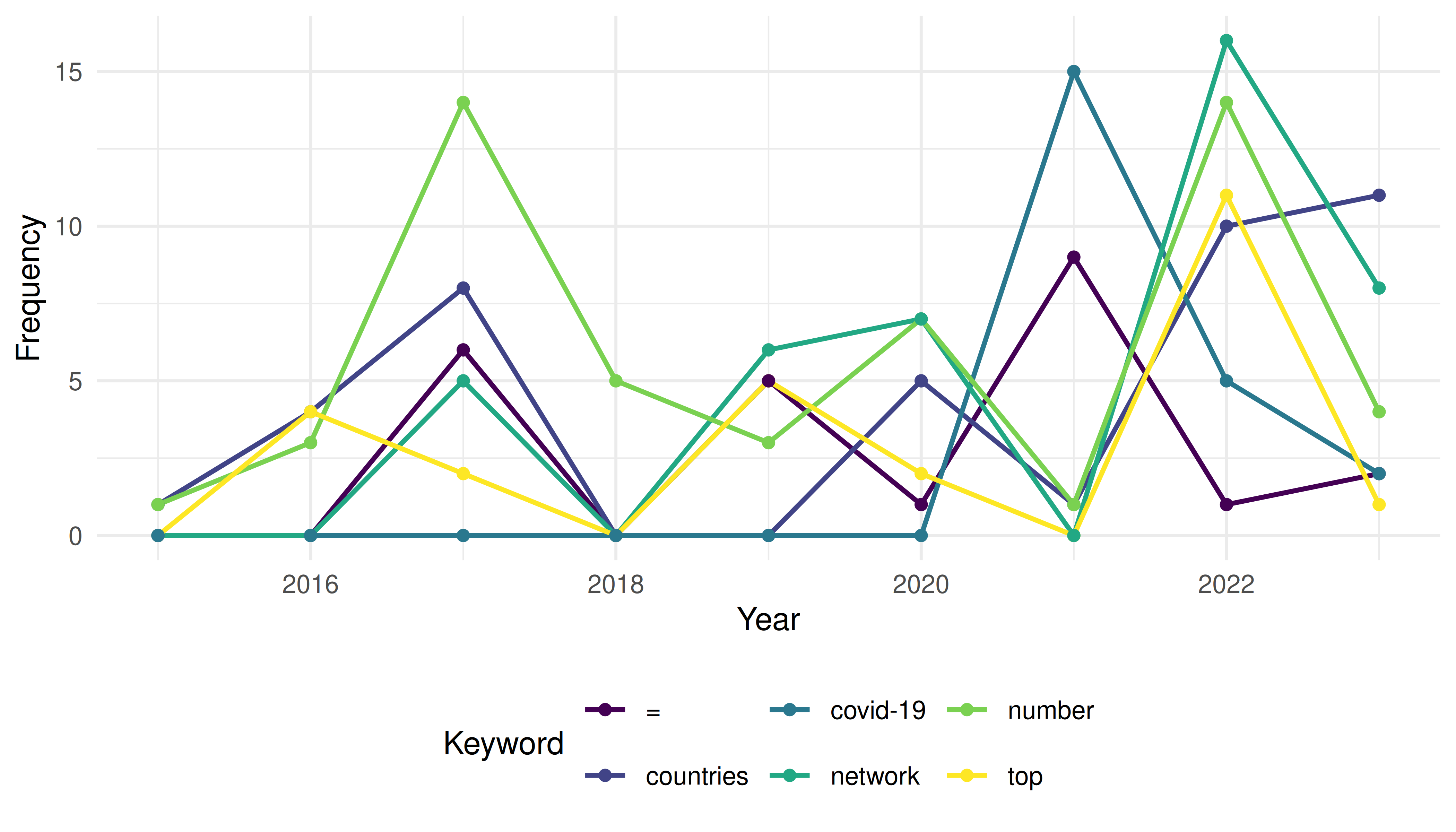

Figure 43.2: Temporal trajectories of selected emerging keywords.

43.6 Topic modelling

dtm <- quanteda::convert(dfmat, to = "topicmodels")
lda <- LDA(dtm, k = 8, control = list(seed = 42))

lda_topics <- tidy(lda, matrix = "beta") |>
  group_by(topic) |>
  slice_max(beta, n = 8) |>
  ungroup()

lda_topics |>
  mutate(term = reorder_within(term, beta, topic)) |>
  ggplot(aes(x = beta, y = term, fill = factor(topic))) +
  geom_col(show.legend = FALSE) +
  facet_wrap(~ paste("Topic", topic), scales = "free_y", ncol = 4) +
  scale_y_reordered() +
  scale_fill_manual(values = palette_sci(8)) +
  labs(x = "Word probability", y = NULL) +
  theme_sci(base_size = 9)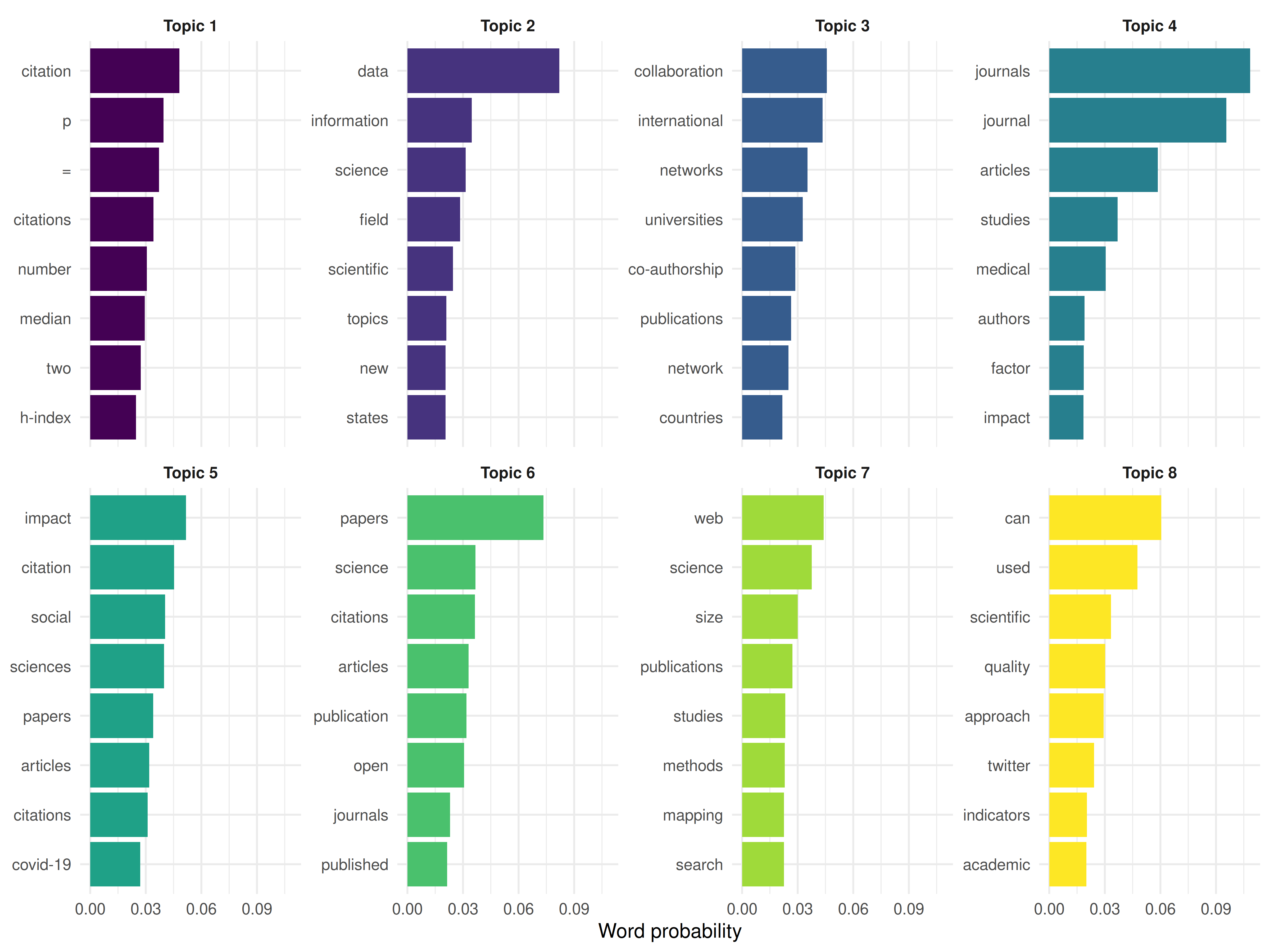

Figure 43.3: Top terms per LDA topic.

43.7 Topic prevalence by year

doc_topics <- tidy(lda, matrix = "gamma") |>
  left_join(text_df |> transmute(document = doc_id, year), by = "document")

topic_by_year <- doc_topics |>
  group_by(year, topic) |>
  summarise(mean_gamma = mean(gamma), .groups = "drop")

ggplot(topic_by_year, aes(x = year, y = mean_gamma, colour = factor(topic))) +
  geom_line(linewidth = 0.7) +
  scale_colour_manual(values = palette_sci(8)) +
  labs(x = "Year", y = "Mean topic proportion", colour = "Topic") +
  theme_sci()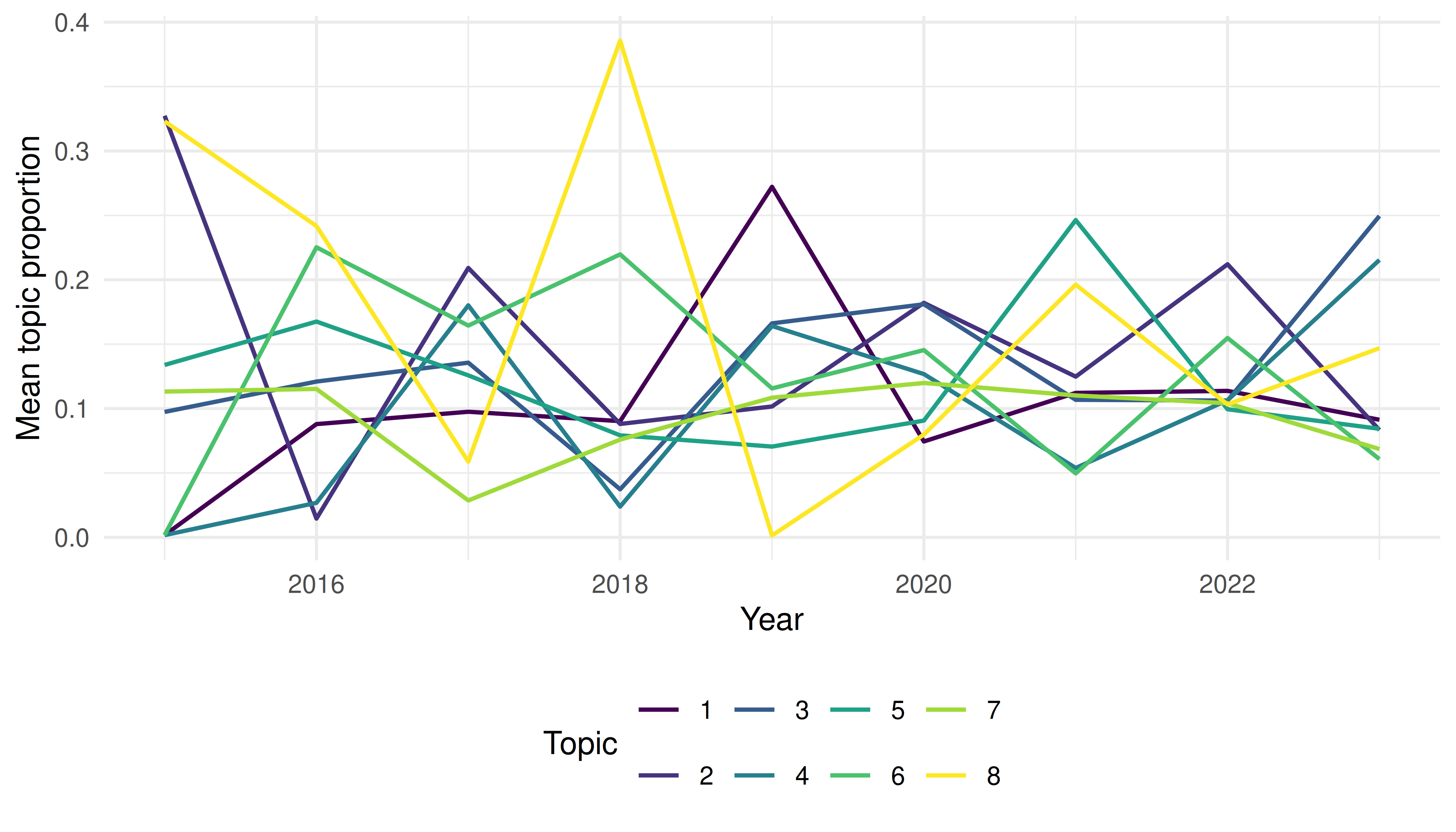

Figure 43.4: Topic prevalence over time.

43.8 Key findings

1. Emerging keywords align with known developments: open science, AI/machine learning applications, equity and diversity, and preprints.
2. Topic evolution shows gradual shifts in emphasis rather than abrupt changes, consistent with a mature field incorporating new tools.
3. Growth rates should be interpreted cautiously: terms with low baseline frequencies can show high percentage growth from small increases.
4. Validation: the topics identified by LDA correspond to recognisable subfields, lending credibility to the unsupervised approach.

43.9 Lessons learned

• Combining keyword growth rates with topic models provides complementary perspectives: growth rates capture individual terms, while topics capture thematic clusters.
• Database coverage growth can create artefactual “emergence.” Always normalise by total corpus size.
• Emerging topics in scientometrics mirror broader trends in science policy (open access mandates, equity initiatives, AI adoption) (Kleinberg 2003).