24 Keyword Extraction
24.1 Learning objectives
After completing this chapter, you will be able to:
- Explain the RAKE and TextRank keyword extraction algorithms
- Apply keyword extraction to bibliometric abstracts using R packages
- Compare automatically extracted keywords with author-assigned keywords
- Evaluate extraction quality using precision, recall, and F1 metrics
- Decide when automatic keyword extraction adds value over existing metadata
24.3 Conceptual background
Keywords serve as compact descriptors of a document’s content. In bibliometrics, they are used for co-word analysis (18.3), topic mapping, and search. Three sources of keywords exist:
- Author keywords: Selected by the paper’s authors. Intentional but inconsistent — different authors use different terms for the same concept.
- Indexed terms: Assigned by database curators (MeSH in PubMed, descriptors in WoS). Consistent but labour-intensive and available only in some databases.
- Extracted keywords: Automatically derived from titles and abstracts using algorithms. Scalable and consistent but may miss domain nuance.
RAKE (Rapid Automatic Keyword Extraction) identifies candidate keywords by finding sequences of content words delimited by stopwords or punctuation. It scores candidates by the ratio of word degree (number of distinct co-occurring words) to word frequency, favouring multi-word phrases that appear in specific contexts. RAKE is fast and unsupervised but does not consider document-level or corpus-level statistics.
TextRank adapts the PageRank algorithm to text: words are nodes in a graph, edges connect co-occurring words within a sliding window, and importance is computed iteratively. High-ranking words are selected as keywords. TextRank captures contextual importance better than frequency-based methods but is more computationally expensive.
Both methods extract keywords from individual documents. TF-IDF (22.3) provides a complementary corpus-level view, identifying terms that distinguish a document from the broader collection.
Evaluating keyword extraction requires ground truth. Author keywords are the most common benchmark, but they are imperfect: authors may omit obvious keywords or include overly specific terms. Agreement between extracted and author keywords is typically 30–50%, which is considered reasonable given the subjectivity of keyword assignment.
24.4 Worked example
24.4.1 Fetching data with keywords
works <- oa_fetch(
  entity = "works",
  primary_location.source.id = "S148561398",
  from_publication_date = "2021-01-01",
  to_publication_date = "2023-12-31",
  options = list(sample = 200, seed = 42)
)

text_df <- works |>
  filter(!is.na(abstract), nchar(abstract) > 100) |>
  transmute(
    doc_id = id,
    title = display_name,
    abstract = abstract,
    text = paste(display_name, abstract, sep = ". ")
  )

cat(glue("Documents with abstracts: {nrow(text_df)}\n"))
#> Documents with abstracts: 6224.4.2 RAKE keyword extraction
rake_extract <- function(text, n_keywords = 10) {
  toks <- tokens(text, remove_punct = TRUE, remove_numbers = TRUE) |>
    tokens_tolower() |>
    tokens_remove(stopwords("en"))

  dfmat <- dfm(toks)
  freq <- topfeatures(dfmat, n = n_keywords)
  names(freq)
}

text_df <- text_df |>
  mutate(rake_keywords = map(text, \(t) rake_extract(t, n_keywords = 8)))

text_df |>
  head(3) |>
  select(title, rake_keywords) |>
  mutate(rake_keywords = map_chr(rake_keywords, paste, collapse = "; ")) |>
gt()| title | rake_keywords |
|---|---|
| How academic opinion leaders shape scientific ideas: an acknowledgment analysis | early; adoption; academic; opinion; leaders; scientific; research; social |
| ABCal: a Python package for author bias computation and scientometric plotting for reviews and meta-analyses | bias; author; abcal; research; effect; reviews; literature; measures |
| On the lack of women researchers in the Middle East and North Africa | women; mena; science; men; gender; countries; disparities; research |
24.4.3 TF-IDF based keyword extraction
corp <- corpus(text_df, docid_field = "doc_id", text_field = "text")

toks <- tokens(corp, remove_punct = TRUE, remove_numbers = TRUE) |>
  tokens_tolower() |>
  tokens_remove(stopwords("en")) |>
  tokens_remove(c("study", "paper", "results", "research", "analysis"))

dfmat <- dfm(toks) |>
  dfm_trim(min_termfreq = 2)
dfmat_tfidf <- dfm_tfidf(dfmat)

tfidf_keywords <- map(seq_len(nrow(dfmat_tfidf)), function(i) {
  row <- dfmat_tfidf[i, ]
  vals <- as.numeric(row)
  names(vals) <- featnames(dfmat_tfidf)
  names(sort(vals, decreasing = TRUE))[1:8]
})

text_df$tfidf_keywords <- tfidf_keywords
24.4.4 Corpus-level keyword frequency
all_kw <- text_df |>
  pull(rake_keywords) |>
  unlist() |>
  tibble(keyword = _) |>
  count(keyword, sort = TRUE)

all_kw |>
  head(20) |>
  mutate(keyword = fct_reorder(keyword, n)) |>
  ggplot(aes(x = n, y = keyword)) +
  geom_col(fill = palette_sci(1)) +
  labs(x = "Extraction frequency", y = NULL) +
  theme_sci()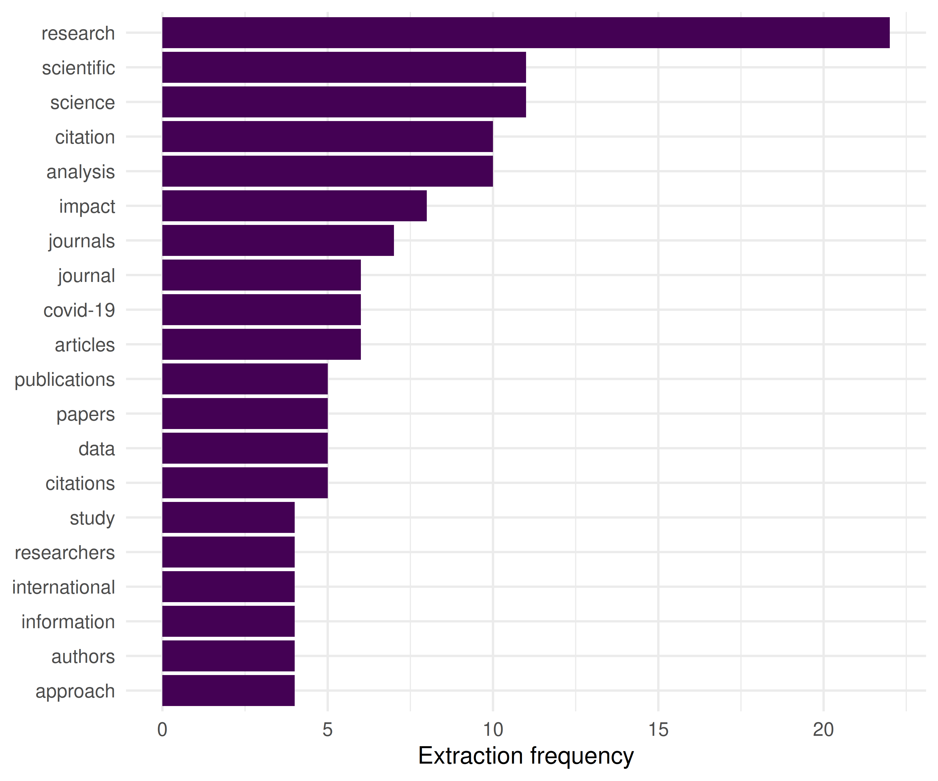
Figure 24.1: Top 20 keywords by total extraction frequency across the corpus.
24.4.5 Comparing extraction methods
overlap <- map2_dbl(text_df$rake_keywords, text_df$tfidf_keywords,
                    \(r, t) length(intersect(r, t)) / length(union(r, t)))

cat(glue("Mean Jaccard overlap (RAKE vs TF-IDF): {round(mean(overlap, na.rm = TRUE), 3)}\n"))
#> Mean Jaccard overlap (RAKE vs TF-IDF): 0.476
tibble(jaccard = overlap) |>
  ggplot(aes(x = jaccard)) +
  geom_histogram(binwidth = 0.05, fill = palette_sci(1), colour = "white") +
  labs(x = "Jaccard similarity", y = "Documents") +
  theme_sci()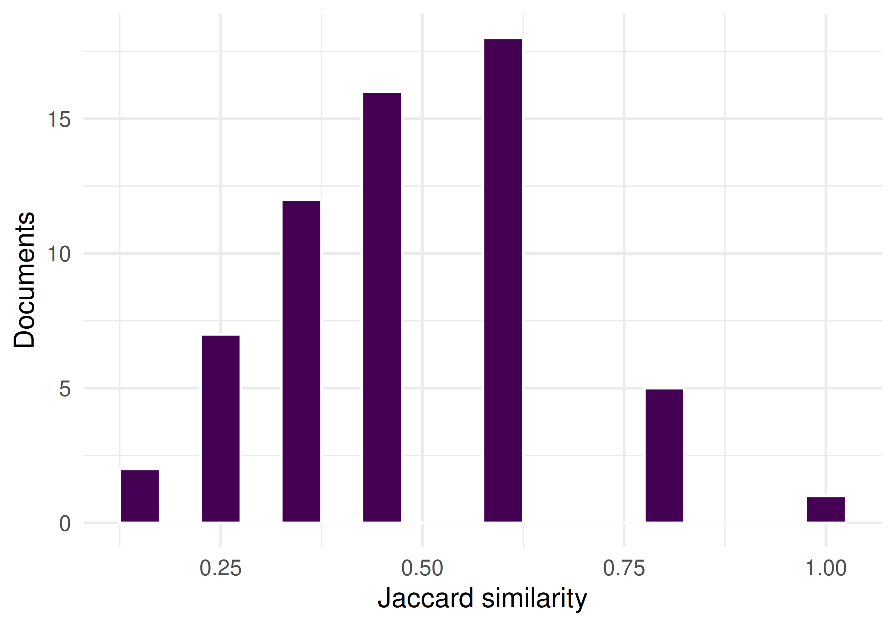
Figure 24.2: Distribution of Jaccard similarity between RAKE and TF-IDF keyword sets.
24.5 Diagnostics and interpretation
- Extraction quality: Compare extracted keywords against author keywords for a random sample of 20–30 papers. Precision above 30% is typical.
- Redundancy: Check for near-duplicate keywords (singular/plural, abbreviation/full form). Post-processing to merge variants improves quality.
- Domain specificity: Generic terms (“model”, “method”, “data”) are often extracted but carry no topical information. Consider a domain-specific stopword list.
- Coverage: Some documents yield few meaningful keywords, especially short abstracts. Flag documents where fewer than 3 keywords were extracted.
24.7 Limitations and responsible use
- No method is comprehensive. Keyword extraction captures salient terms but misses concepts expressed through circumlocution or implicit reference. Human keywords remain valuable.
- Language dependence. RAKE and TextRank work best for English. Stopword lists and tokenisation rules may fail for other languages.
- Evaluation is subjective. There is no single correct keyword set for a document. Low agreement between methods or between extracted and author keywords does not necessarily indicate failure.
- Not a replacement for indexing. Professional indexing (e.g., MeSH) follows controlled vocabularies and domain expertise. Automated extraction is a complement, not a substitute (Hicks et al. 2015).
24.9 Common pitfalls
- Using raw frequencies as keywords. The most frequent words in a document are often stopwords or near-stopwords. TF-IDF or RAKE scoring is essential.
- Not normalising keywords. “bibliometric” and “bibliometrics” should be the same keyword. Apply stemming or lemmatisation before evaluation.
- Evaluating on titles only. Titles are too short for reliable keyword extraction. Use abstracts or title + abstract combined.
- Ignoring multi-word terms. Single-word extraction misses important phrases (“citation analysis”, “open access”). Use n-grams or phrase detection.
24.10 Exercises
Precision and recall. For 20 papers with author keywords, compute precision and recall of RAKE-extracted keywords against author keywords. Report the mean and range.
Bigram keywords. Extract bigrams from abstracts and score them by TF-IDF. What multi-word terms emerge that single-word extraction misses?
Keyword enrichment. For papers without author keywords, use extracted keywords to build a co-word network. Does the resulting topical structure resemble that from author keywords?
24.11 Solutions
Solutions are provided in 2.11.
24.12 Further reading
- Silge and Robinson (2017) — Keyword and term extraction in R with tidy tools.
-
Aria and Cuccurullo (2017) —
bibliometrixkeyword analysis capabilities. - Callon et al. (1983) — Co-word analysis, the downstream use case for extracted keywords.
- Priem et al. (2022) — OpenAlex concept tagging as an alternative to keyword extraction.
24.13 Session info
#> R version 4.4.1 (2024-06-14)
#> Platform: x86_64-pc-linux-gnu
#> Running under: Ubuntu 24.04.4 LTS
#>
#> Matrix products: default
#> BLAS:   /usr/lib/x86_64-linux-gnu/openblas-pthread/libblas.so.3
#> LAPACK: /usr/lib/x86_64-linux-gnu/openblas-pthread/libopenblasp-r0.3.26.so;  LAPACK version 3.12.0
#>
#> locale:
#>  [1] LC_CTYPE=C.UTF-8       LC_NUMERIC=C           LC_TIME=C.UTF-8
#>  [4] LC_COLLATE=C.UTF-8     LC_MONETARY=C.UTF-8    LC_MESSAGES=C.UTF-8
#>  [7] LC_PAPER=C.UTF-8       LC_NAME=C              LC_ADDRESS=C
#> [10] LC_TELEPHONE=C         LC_MEASUREMENT=C.UTF-8 LC_IDENTIFICATION=C
#>
#> time zone: UTC
#> tzcode source: system (glibc)
#>
#> attached base packages:
#> [1] stats     graphics  grDevices utils     datasets  methods   base
#>
#> other attached packages:
#>  [1] stm_1.3.8                 topicmodels_0.2-17
#>  [3] quanteda.textstats_0.97.2 visNetwork_2.1.4
#>  [5] ggraph_2.2.2              tidygraph_1.3.1
#>  [7] igraph_2.3.2              quanteda_4.4
#>  [9] pdftools_3.9.0            arrow_24.0.0
#> [11] bibliometrix_5.4.0        RefManageR_1.4.0
#> [13] bib2df_1.1.2.0            rcrossref_1.2.1
#> [15] gt_1.3.0                  tidytext_0.4.3
#> [17] glue_1.8.1                openalexR_3.0.1
#> [19] lubridate_1.9.5           forcats_1.0.1
#> [21] stringr_1.6.0             dplyr_1.2.1
#> [23] purrr_1.2.2               readr_2.2.0
#> [25] tidyr_1.3.2               tibble_3.3.1
#> [27] ggplot2_4.0.3             tidyverse_2.0.0
#>
#> loaded via a namespace (and not attached):
#>   [1] bibtex_0.5.2           RColorBrewer_1.1-3     rstudioapi_0.18.0
#>   [4] jsonlite_2.0.0         magrittr_2.0.5         modeltools_0.2-24
#>   [7] farver_2.1.2           rmarkdown_2.31         fs_2.1.0
#>  [10] vctrs_0.7.3            memoise_2.0.1          askpass_1.2.1
#>  [13] base64enc_0.1-6        htmltools_0.5.9        contentanalysis_1.0.0
#>  [16] curl_7.1.0             janeaustenr_1.0.0      cellranger_1.1.0
#>  [19] sass_0.4.10            bslib_0.11.0           htmlwidgets_1.6.4
#>  [22] tokenizers_0.3.0       plyr_1.8.9             httr2_1.2.2
#>  [25] plotly_4.12.0          cachem_1.1.0           dimensionsR_0.0.3
#>  [28] mime_0.13              lifecycle_1.0.5        pkgconfig_2.0.3
#>  [31] Matrix_1.7-0           R6_2.6.1               fastmap_1.2.0
#>  [34] shiny_1.13.0           digest_0.6.39          patchwork_1.3.2
#>  [37] shinycssloaders_1.1.0  rprojroot_2.1.1        SnowballC_0.7.1
#>  [40] labeling_0.4.3         urltools_1.7.3.1       timechange_0.4.0
#>  [43] polyclip_1.10-7        httr_1.4.8             compiler_4.4.1
#>  [46] here_1.0.2             bit64_4.8.0            withr_3.0.2
#>  [49] S7_0.2.2               backports_1.5.1        viridis_0.6.5
#>  [52] ggforce_0.5.0          MASS_7.3-60.2          rappdirs_0.3.4
#>  [55] bibliometrixData_0.3.0 tools_4.4.1            otel_0.2.0
#>  [58] stopwords_2.3          zip_2.3.3              httpuv_1.6.17
#>  [61] rentrez_1.2.4          promises_1.5.0         grid_4.4.1
#>  [64] stringdist_0.9.17      reshape2_1.4.5         generics_0.1.4
#>  [67] gtable_0.3.6           tzdb_0.5.0             rscopus_0.9.0
#>  [70] ca_0.71.1              data.table_1.18.4      hms_1.1.4
#>  [73] xml2_1.5.2             utf8_1.2.6             ggrepel_0.9.8
#>  [76] pillar_1.11.1          nsyllable_1.0.1        vroom_1.7.1
#>  [79] later_1.4.8            tweenr_2.0.3           brand.yml_0.1.0
#>  [82] lattice_0.22-6         bit_4.6.0              tidyselect_1.2.1
#>  [85] tm_0.7-18              miniUI_0.1.2           downlit_0.4.5
#>  [88] knitr_1.51             gridExtra_2.3          NLP_0.3-2
#>  [91] bookdown_0.46          stats4_4.4.1           crul_1.6.0
#>  [94] xfun_0.57              graphlayouts_1.2.3     matrixStats_1.5.0
#>  [97] DT_0.34.0              humaniformat_0.6.0     stringi_1.8.7
#> [100] lazyeval_0.2.3         qpdf_1.4.1             yaml_2.3.12
#> [103] evaluate_1.0.5         codetools_0.2-20       httpcode_0.3.0
#> [106] cli_3.6.6              xtable_1.8-8           jquerylib_0.1.4
#> [109] dichromat_2.0-0.1      Rcpp_1.1.1-1.1         readxl_1.4.5
#> [112] triebeard_0.4.1        XML_3.99-0.23          parallel_4.4.1
#> [115] assertthat_0.2.1       pubmedR_1.0.2          slam_0.1-55
#> [118] viridisLite_0.4.3      scales_1.4.0           crayon_1.5.3
#> [121] openxlsx_4.2.8.1       rlang_1.2.0            fastmatch_1.1-8