33 Causal Inference in Scientometrics
33.1 Learning objectives
After completing this chapter, you will be able to:
- Distinguish causal from correlational claims in bibliometric research
- Apply difference-in-differences to evaluate the effect of a policy change
- Use propensity score matching to create comparable treatment and control groups
- Interpret regression discontinuity designs for threshold-based interventions
- Recognise the assumptions underlying causal inference in observational bibliometric data
33.3 Conceptual background
Bibliometrics is rich in correlations: OA papers are more cited than closed-access papers; funded research receives more citations; papers in prestigious journals are cited more. But correlation does not imply causation. The OA citation advantage may reflect self-selection (better papers are more likely to be made OA), not the causal effect of open access. Separating cause from confound is essential for evidence-based science policy.
Difference-in-differences (DiD) exploits policy changes as natural experiments. If a funder mandates OA starting in year T, papers from that funder before and after T serve as the treatment group, while papers from a similar funder without the mandate serve as the control. The causal effect is estimated as the difference in trends between treatment and control groups. The key assumption is parallel trends: absent the intervention, both groups would have followed the same trajectory.
Regression discontinuity design (RDD) applies when treatment is assigned by a threshold. For example, grants are funded above a score cutoff; papers are accepted above a review score threshold. Comparing outcomes just above and just below the threshold isolates the causal effect of the treatment, under the assumption that units near the threshold are comparable.
Matching methods create comparable groups from observational data. Propensity score matching pairs treated units (e.g., OA papers) with control units (closed-access papers) that have similar observable characteristics (field, journal, year, team size). This reduces confounding but cannot eliminate unmeasured confounders.
All three methods require strong assumptions. In bibliometrics, violations are common: the parallel trends assumption may fail because of concurrent policy changes; the RDD threshold may be manipulable; matching cannot address unmeasured confounders like paper quality. Hicks et al. (2015) emphasise that quantitative analysis, however sophisticated, cannot replace expert judgement in research evaluation.
33.4 Worked example
33.4.1 Setting up a DiD analysis: OA status and citations
works <- oa_fetch(
  entity = "works",
  primary_location.source.id = "S148561398",
  from_publication_date = "2016-01-01",
  to_publication_date = "2023-12-31",
  type = "article",
  options = list(sample = 500, seed = 42)
)

did_data <- works |>
  transmute(
    id, year = year(publication_date),
    cited_by_count,
    is_oa = oa_status != "closed",
    post_2020 = year >= 2020,
    referenced_works_count
  )

cat(glue("Papers: {nrow(did_data)}\n"))
#> Papers: 500#> OA: 207, Closed: 29333.4.2 Descriptive comparison
did_summary <- did_data |>
  group_by(is_oa, post_2020) |>
  summarise(mean_cites = mean(cited_by_count), n = n(), .groups = "drop") |>
  mutate(period = ifelse(post_2020, "2020-2023", "2016-2019"),
         group = ifelse(is_oa, "Open access", "Closed"))

ggplot(did_summary, aes(x = period, y = mean_cites, fill = group)) +
  geom_col(position = "dodge") +
  scale_fill_manual(values = palette_sci(2)) +
  labs(x = "Period", y = "Mean citations", fill = "Access") +
  theme_sci()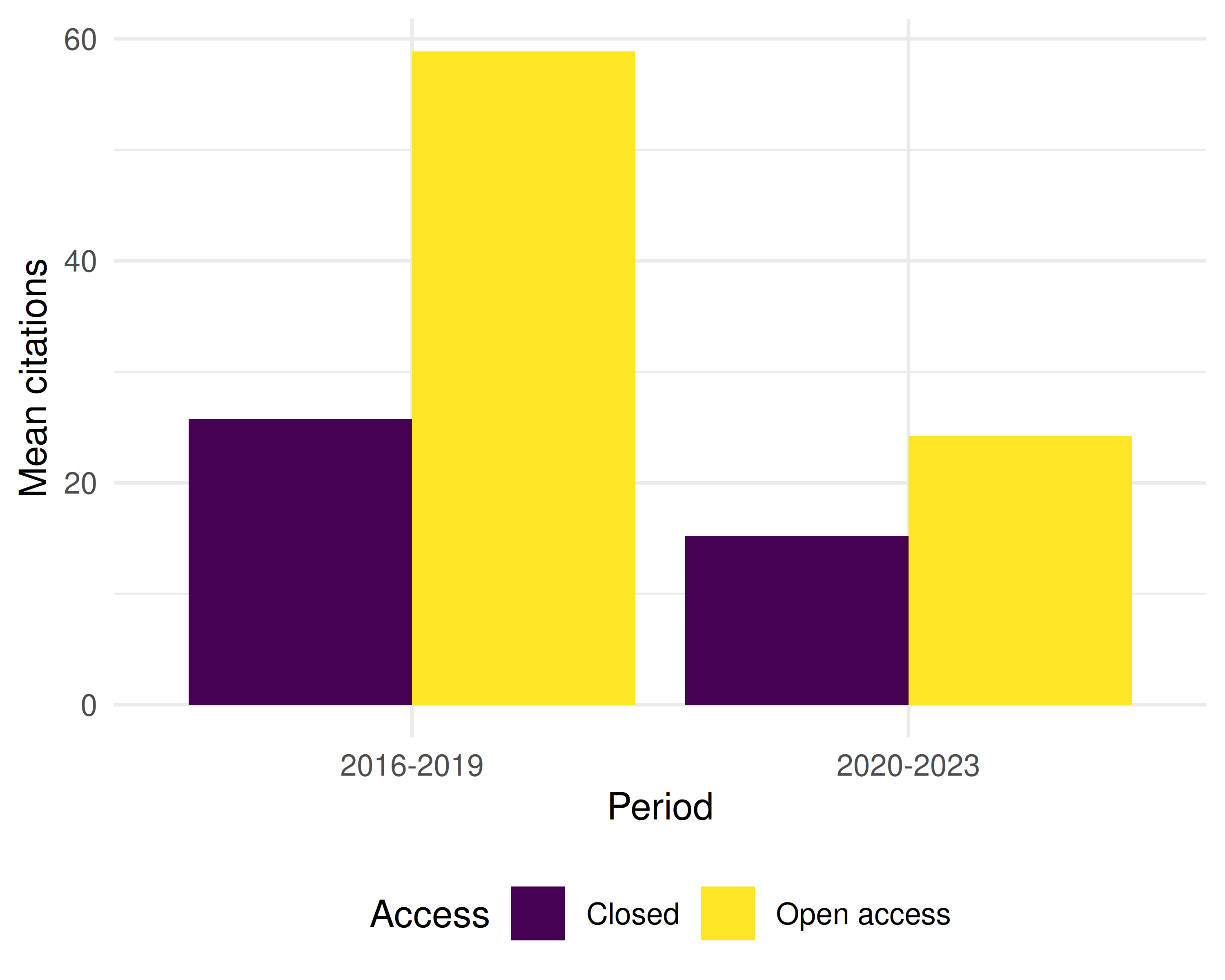
Figure 33.1: Mean citations by OA status and time period.
33.4.3 DiD regression
did_model <- lm(cited_by_count ~ is_oa * post_2020 + referenced_works_count,
                data = did_data)

tidy_did <- broom::tidy(did_model)
tidy_did |>
  mutate(across(where(is.numeric), \(x) round(x, 3))) |>
gt()| term | estimate | std.error | statistic | p.value |
|---|---|---|---|---|
| (Intercept) | 20.163 | 3.204 | 6.29 | 0.000 |
| is_oaTRUE | 18.375 | 3.977 | 4.62 | 0.000 |
| post_2020TRUE | -13.082 | 3.598 | -3.64 | 0.000 |
| referenced_works_count | 0.149 | 0.047 | 3.15 | 0.002 |
| is_oaTRUE:post_2020TRUE | -11.609 | 5.571 | -2.08 | 0.038 |
33.4.4 Simple matching comparison
oa_papers <- did_data |> filter(is_oa)
closed_papers <- did_data |> filter(!is_oa)

matched <- oa_papers |>
  mutate(match_year = year) |>
  inner_join(
    closed_papers |> select(year, cited_by_count_closed = cited_by_count),
    by = "year",
    relationship = "many-to-many"
  ) |>
  group_by(id) |>
  slice_sample(n = 1) |>
  ungroup()

cat(glue("Matched pairs: {nrow(matched)}\n"))
#> Matched pairs: 207#> Mean cites (OA): 31.4#> Mean cites (closed match): 24.533.4.5 Visualising the parallel trends assumption
trends <- did_data |>
  group_by(year, is_oa) |>
  summarise(mean_cites = mean(cited_by_count), .groups = "drop") |>
  mutate(group = ifelse(is_oa, "OA", "Closed"))

ggplot(trends, aes(x = year, y = mean_cites, colour = group)) +
  geom_line(linewidth = 1) +
  geom_point(size = 2) +
  geom_vline(xintercept = 2019.5, linetype = "dashed", colour = "grey50") +
  scale_colour_manual(values = palette_sci(2)) +
  labs(x = "Year", y = "Mean citations", colour = "Access") +
  theme_sci()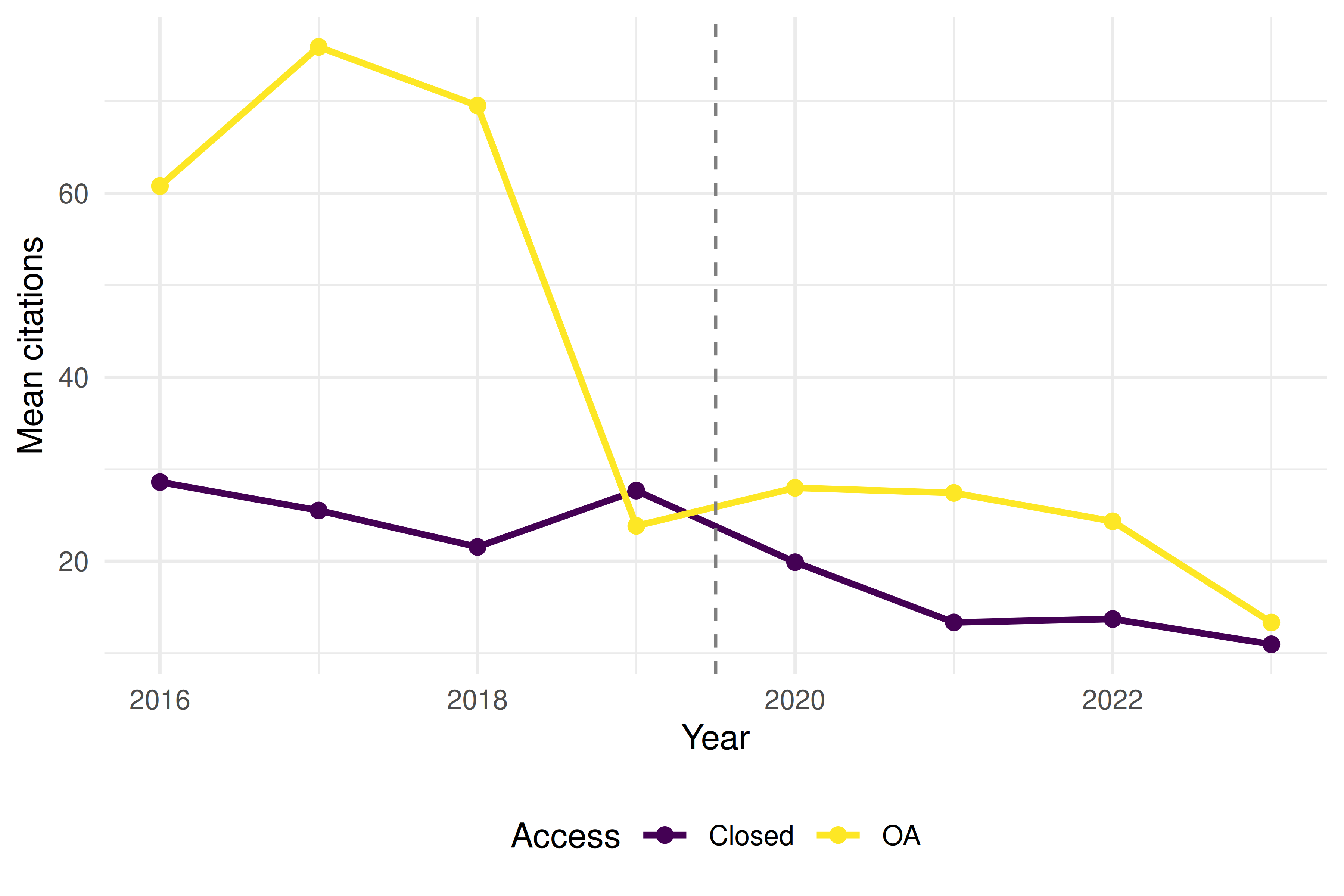
Figure 33.2: Citation trends by OA status over time (checking parallel trends).
33.5 Diagnostics and interpretation
- Parallel trends: Inspect pre-treatment trends visually. If OA and closed papers had diverging trends before 2020, the DiD estimate is biased.
- Covariate balance: After matching, check that matched pairs have similar observable characteristics (year, reference count, journal).
- Effect size interpretation: A statistically significant DiD coefficient does not mean the effect is practically important. Report effect sizes alongside p-values.
- Robustness checks: Run the analysis with different control groups, time windows, and matching criteria. Consistent results increase confidence.
33.7 Limitations and responsible use
- Observational data cannot prove causation. All causal inference methods applied to bibliometric data make assumptions that cannot be fully tested. Report assumptions explicitly.
- Unmeasured confounders. Paper quality, author reputation, and marketing effort are rarely observable in bibliometric data but strongly affect citations.
- Treatment definition. “OA” is not a single treatment — it encompasses gold, green, hybrid, and bronze, each with different mechanisms.
- Generalisability. Causal estimates from one journal, field, or time period may not generalise to others.
- Policy implications require judgement. Even a well-estimated causal effect is one input into policy decisions, not a sufficient basis for mandates (Hicks et al. 2015; American Society for Cell Biology 2012).
33.9 Common pitfalls
- Claiming causation from regression coefficients. A positive OA coefficient in a regression does not prove OA causes more citations without addressing confounders.
- Ignoring parallel trends violations. If pre-treatment trends are not parallel, DiD estimates are biased. Do not ignore this in reporting.
- Matching on too few covariates. Matching on year alone leaves many confounders unaddressed. Include as many relevant covariates as possible.
- Over-interpreting p-values. A p < 0.05 does not mean the result is practically significant or that the causal assumptions hold.
33.10 Exercises
Extended DiD. Add additional covariates (document type, number of authors) to the DiD regression. Does the OA interaction term change?
Placebo test. Run the DiD analysis using 2018 as the treatment year instead of 2020. If the interaction term is significant, the parallel trends assumption may be violated.
Matched comparison. Implement propensity score matching (using the
MatchItpackage) with year, reference count, and document type as covariates. Compare the matched OA effect to the unmatched effect.
33.11 Solutions
Solutions are provided in 2.11.
33.13 Session info
#> R version 4.4.1 (2024-06-14)
#> Platform: x86_64-pc-linux-gnu
#> Running under: Ubuntu 24.04.4 LTS
#>
#> Matrix products: default
#> BLAS:   /usr/lib/x86_64-linux-gnu/openblas-pthread/libblas.so.3
#> LAPACK: /usr/lib/x86_64-linux-gnu/openblas-pthread/libopenblasp-r0.3.26.so;  LAPACK version 3.12.0
#>
#> locale:
#>  [1] LC_CTYPE=C.UTF-8       LC_NUMERIC=C           LC_TIME=C.UTF-8
#>  [4] LC_COLLATE=C.UTF-8     LC_MONETARY=C.UTF-8    LC_MESSAGES=C.UTF-8
#>  [7] LC_PAPER=C.UTF-8       LC_NAME=C              LC_ADDRESS=C
#> [10] LC_TELEPHONE=C         LC_MEASUREMENT=C.UTF-8 LC_IDENTIFICATION=C
#>
#> time zone: UTC
#> tzcode source: system (glibc)
#>
#> attached base packages:
#> [1] stats     graphics  grDevices utils     datasets  methods   base
#>
#> other attached packages:
#>  [1] uwot_0.2.4                Matrix_1.7-0
#>  [3] word2vec_0.4.1            stm_1.3.8
#>  [5] topicmodels_0.2-17        quanteda.textstats_0.97.2
#>  [7] visNetwork_2.1.4          ggraph_2.2.2
#>  [9] tidygraph_1.3.1           igraph_2.3.2
#> [11] quanteda_4.4              pdftools_3.9.0
#> [13] arrow_24.0.0              bibliometrix_5.4.0
#> [15] RefManageR_1.4.0          bib2df_1.1.2.0
#> [17] rcrossref_1.2.1           gt_1.3.0
#> [19] tidytext_0.4.3            glue_1.8.1
#> [21] openalexR_3.0.1           lubridate_1.9.5
#> [23] forcats_1.0.1             stringr_1.6.0
#> [25] dplyr_1.2.1               purrr_1.2.2
#> [27] readr_2.2.0               tidyr_1.3.2
#> [29] tibble_3.3.1              ggplot2_4.0.3
#> [31] tidyverse_2.0.0
#>
#> loaded via a namespace (and not attached):
#>   [1] bibtex_0.5.2           RColorBrewer_1.1-3     rstudioapi_0.18.0
#>   [4] jsonlite_2.0.0         magrittr_2.0.5         modeltools_0.2-24
#>   [7] farver_2.1.2           rmarkdown_2.31         fs_2.1.0
#>  [10] vctrs_0.7.3            memoise_2.0.1          askpass_1.2.1
#>  [13] base64enc_0.1-6        htmltools_0.5.9        contentanalysis_1.0.0
#>  [16] curl_7.1.0             broom_1.0.12           janeaustenr_1.0.0
#>  [19] cellranger_1.1.0       sass_0.4.10            bslib_0.11.0
#>  [22] htmlwidgets_1.6.4      tokenizers_0.3.0       plyr_1.8.9
#>  [25] httr2_1.2.2            plotly_4.12.0          cachem_1.1.0
#>  [28] dimensionsR_0.0.3      mime_0.13              lifecycle_1.0.5
#>  [31] pkgconfig_2.0.3        R6_2.6.1               fastmap_1.2.0
#>  [34] shiny_1.13.0           digest_0.6.39          patchwork_1.3.2
#>  [37] shinycssloaders_1.1.0  rprojroot_2.1.1        RSpectra_0.16-2
#>  [40] SnowballC_0.7.1        labeling_0.4.3         urltools_1.7.3.1
#>  [43] timechange_0.4.0       mgcv_1.9-1             polyclip_1.10-7
#>  [46] httr_1.4.8             compiler_4.4.1         here_1.0.2
#>  [49] bit64_4.8.0            withr_3.0.2            S7_0.2.2
#>  [52] backports_1.5.1        viridis_0.6.5          ggforce_0.5.0
#>  [55] MASS_7.3-60.2          rappdirs_0.3.4         bibliometrixData_0.3.0
#>  [58] tools_4.4.1            otel_0.2.0             stopwords_2.3
#>  [61] zip_2.3.3              httpuv_1.6.17          rentrez_1.2.4
#>  [64] nlme_3.1-164           promises_1.5.0         grid_4.4.1
#>  [67] stringdist_0.9.17      reshape2_1.4.5         generics_0.1.4
#>  [70] gtable_0.3.6           tzdb_0.5.0             rscopus_0.9.0
#>  [73] ca_0.71.1              data.table_1.18.4      hms_1.1.4
#>  [76] xml2_1.5.2             utf8_1.2.6             ggrepel_0.9.8
#>  [79] pillar_1.11.1          nsyllable_1.0.1        vroom_1.7.1
#>  [82] later_1.4.8            splines_4.4.1          tweenr_2.0.3
#>  [85] brand.yml_0.1.0        lattice_0.22-6         FNN_1.1.4.1
#>  [88] bit_4.6.0              tidyselect_1.2.1       tm_0.7-18
#>  [91] miniUI_0.1.2           downlit_0.4.5          knitr_1.51
#>  [94] gridExtra_2.3          NLP_0.3-2              bookdown_0.46
#>  [97] stats4_4.4.1           crul_1.6.0             xfun_0.57
#> [100] graphlayouts_1.2.3     matrixStats_1.5.0      DT_0.34.0
#> [103] humaniformat_0.6.0     stringi_1.8.7          lazyeval_0.2.3
#> [106] qpdf_1.4.1             yaml_2.3.12            evaluate_1.0.5
#> [109] codetools_0.2-20       httpcode_0.3.0         cli_3.6.6
#> [112] xtable_1.8-8           jquerylib_0.1.4        dichromat_2.0-0.1
#> [115] Rcpp_1.1.1-1.1         readxl_1.4.5           triebeard_0.4.1
#> [118] XML_3.99-0.23          parallel_4.4.1         assertthat_0.2.1
#> [121] pubmedR_1.0.2          slam_0.1-55            viridisLite_0.4.3
#> [124] scales_1.4.0           crayon_1.5.3           openxlsx_4.2.8.1
#> [127] rlang_1.2.0            fastmatch_1.1-8