21 Network Visualization and Interoperability
21.1 Learning objectives
After completing this chapter, you will be able to:
- Choose appropriate layout algorithms for different network types
- Export igraph networks to Gephi (GraphML), VOSviewer, and Pajek formats
- Create interactive network visualisations with
visNetwork - Apply colour and size encoding that communicates structure clearly
- Produce publication-quality static network figures with
ggraph
21.3 Conceptual background
Network visualisation is both an analytical tool and a communication device. A well-designed network figure can reveal structure — clusters, bridges, outliers — at a glance. A poorly designed one obscures these patterns in visual noise.
Layout algorithms determine node positions. Force-directed layouts (Fruchterman-Reingold, Kamada-Kawai) simulate physical forces: connected nodes attract, all nodes repel. They work well for small-to-medium networks (up to ~1,000 nodes) and produce aesthetically pleasing results. For larger networks, the DrL (Distributed Recursive Layout) or OpenOrd algorithms scale better. For trees or hierarchies, Reingold-Tilford or Sugiyama layouts are appropriate. The choice of algorithm depends on the network’s structure and the visual question being asked.
Visual encoding maps network properties to visual channels: node size (degree, centrality), node colour (community, attribute), edge width (weight), and edge colour or transparency. Effective encoding follows the principle of proportional ink: the visual weight of an element should correspond to its data importance. Avoid redundant encoding (mapping the same variable to both size and colour) and limit the number of distinct colours to what the reader can distinguish (typically 8–12 categories) (Fortunato 2010).
Interoperability is essential because no single tool excels at everything. R with igraph and ggraph is excellent for reproducible analysis and publication figures. Gephi (Bastian et al. 2009) provides a rich GUI for exploration and layout refinement. VOSviewer specialises in bibliometric network visualisation with built-in clustering. Pajek handles very large networks efficiently. A practical workflow often involves constructing and analysing the network in R, then exporting to a specialised tool for specific visualisation tasks.
Reproducibility requires that layouts are deterministic. Force-directed algorithms start from random positions, so set.seed() before every layout computation. For cross-tool reproducibility, export node coordinates alongside the network data.
21.4 Worked example
21.4.1 Building a sample network
We reuse a co-authorship network from Scientometrics.
works <- oa_fetch(
  entity = "works",
  primary_location.source.id = "S148561398",
  from_publication_date = "2021-01-01",
  to_publication_date = "2023-12-31",
  options = list(sample = 200, seed = 42)
)

author_data <- works |>
  select(id, authorships) |>
  unnest(authorships, names_sep = "_") |>
  select(work_id = id, author_id = authorships_id,
         author_name = authorships_display_name) |>
  filter(!is.na(author_id))

edges <- author_data |>
  inner_join(author_data, by = "work_id", suffix = c("_1", "_2"),
             relationship = "many-to-many") |>
  filter(author_id_1 < author_id_2) |>
  count(author_id_1, author_id_2, name = "weight")

g <- graph_from_data_frame(
  edges |> select(author_id_1, author_id_2, weight),
  directed = FALSE
) |>
  simplify(edge.attr.comb = list(weight = "sum"))

comp <- components(g)
giant <- induced_subgraph(g, which(comp$membership == which.max(comp$csize)))

comm <- cluster_leiden(giant, resolution_parameter = 1.0,
                       objective_function = "modularity")
V(giant)$community <- membership(comm)
V(giant)$degree <- degree(giant)

author_lookup <- author_data |> distinct(author_id, author_name)
V(giant)$label <- author_lookup$author_name[
  match(V(giant)$name, author_lookup$author_id)
]

cat(glue("Network: {vcount(giant)} nodes, {ecount(giant)} edges\n"))
#> Network: 28 nodes, 306 edges21.4.2 Comparing layout algorithms
tg <- as_tbl_graph(giant) |>
  mutate(community = as.factor(community))

layouts <- c("fr", "kk", "stress", "drl")
layout_names <- c("Fruchterman-Reingold", "Kamada-Kawai", "Stress", "DrL")

plots <- map2(layouts, layout_names, function(algo, name) {
  set.seed(42)
  ggraph(tg, layout = algo) +
    geom_edge_link(alpha = 0.1, colour = "grey60") +
    geom_node_point(aes(colour = community, size = degree), alpha = 0.7) +
    scale_size_continuous(range = c(0.5, 4), guide = "none") +
    scale_colour_manual(values = palette_sci(
      n_distinct(V(giant)$community)
    ), guide = "none") +
    labs(title = name) +
    theme_void(base_family = "sans", base_size = 11)
})

patchwork::wrap_plots(plots, ncol = 2)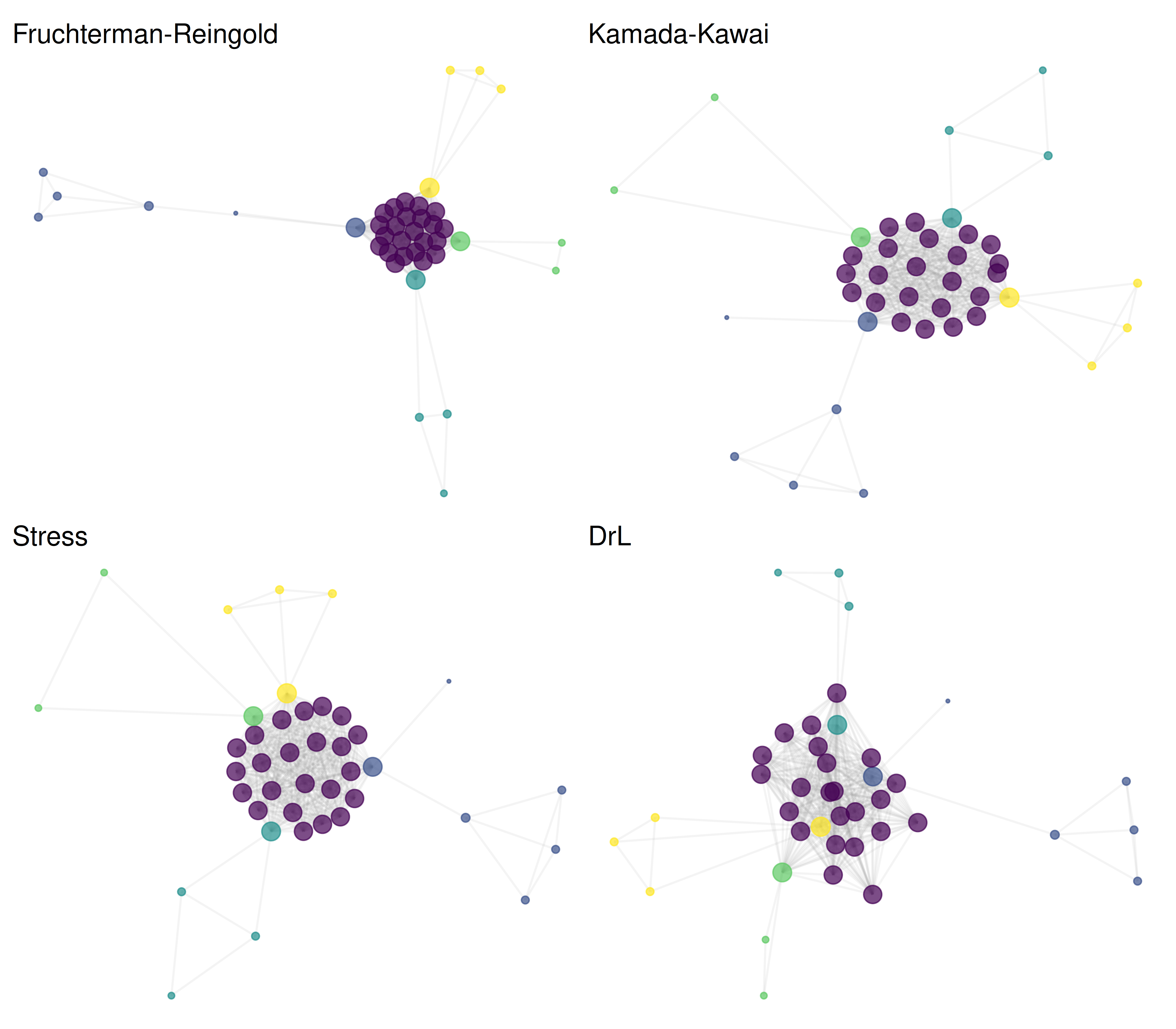
Figure 21.1: The same network rendered with four different layout algorithms.
21.4.3 Exporting to GraphML (Gephi)
out_dir <- here::here("data")
graphml_path <- file.path(out_dir, "coauth_network.graphml")
write_graph(giant, graphml_path, format = "graphml")
cat(glue("Exported GraphML: {graphml_path}\n"))
#> Exported GraphML: /home/runner/work/scientometrics-in-r/scientometrics-in-r/data/coauth_network.graphml#> File size: 31.8 KB21.4.4 Exporting to Pajek format
pajek_path <- file.path(out_dir, "coauth_network.net")
write_graph(giant, pajek_path, format = "pajek")
cat(glue("Exported Pajek: {pajek_path}\n"))
#> Exported Pajek: /home/runner/work/scientometrics-in-r/scientometrics-in-r/data/coauth_network.net21.4.5 Exporting to VOSviewer format
VOSviewer reads tab-separated map and network files.
set.seed(42)
coords <- layout_with_fr(giant)

vos_map <- tibble(
  id = seq_len(vcount(giant)),
  label = V(giant)$label,
  x = coords[, 1],
  y = coords[, 2],
  cluster = V(giant)$community,
  weight = V(giant)$degree
)

vos_network <- as_data_frame(giant, what = "edges") |>
  mutate(
    from_idx = match(from, V(giant)$name),
    to_idx = match(to, V(giant)$name)
  ) |>
  select(from_idx, to_idx, weight)

map_path <- file.path(out_dir, "vosviewer_map.txt")
net_path <- file.path(out_dir, "vosviewer_network.txt")

write_tsv(vos_map, map_path)
write_tsv(vos_network, net_path)
cat(glue("VOSviewer map: {map_path}\n"))
#> VOSviewer map: /home/runner/work/scientometrics-in-r/scientometrics-in-r/data/vosviewer_map.txt#> VOSviewer network: /home/runner/work/scientometrics-in-r/scientometrics-in-r/data/vosviewer_network.txt21.4.6 Interactive visualisation with visNetwork
# HTML widget — only rendered for HTML output (PDF/EPUB skip this chunk).
vis_nodes <- tibble(
  id = V(giant)$name,
  label = ifelse(V(giant)$degree > quantile(V(giant)$degree, 0.9),
                 V(giant)$label, ""),
  title = paste0(V(giant)$label, "<br>Degree: ", V(giant)$degree,
                 "<br>Community: ", V(giant)$community),
  group = as.character(V(giant)$community),
  value = V(giant)$degree
)

vis_edges <- as_data_frame(giant, what = "edges") |>
  select(from, to, weight = weight)

visNetwork(vis_nodes, vis_edges, width = "100%", height = "500px") |>
  visOptions(highlightNearest = TRUE, nodesIdSelection = TRUE) |>
  visPhysics(stabilization = FALSE) |>
  visLayout(randomSeed = 42)
Figure 21.2: Interactive co-authorship network (zoom, pan, and hover for details).
21.4.7 Publication-quality figure
set.seed(42)

ggraph(tg, layout = "fr") +
  geom_edge_link(alpha = 0.08, colour = "grey60") +
  geom_node_point(aes(size = degree, colour = community), alpha = 0.8) +
  geom_node_text(
    aes(label = ifelse(degree > quantile(degree, 0.95), label, NA)),
    repel = TRUE, size = 2.5, max.overlaps = 15, na.rm = TRUE
  ) +
  scale_size_continuous(range = c(1, 6), guide = "none") +
  scale_colour_manual(values = palette_sci(
    n_distinct(V(giant)$community)
  )) +
  labs(colour = "Community") +
  theme_void(base_family = "sans", base_size = 11) +
  theme(legend.position = "bottom")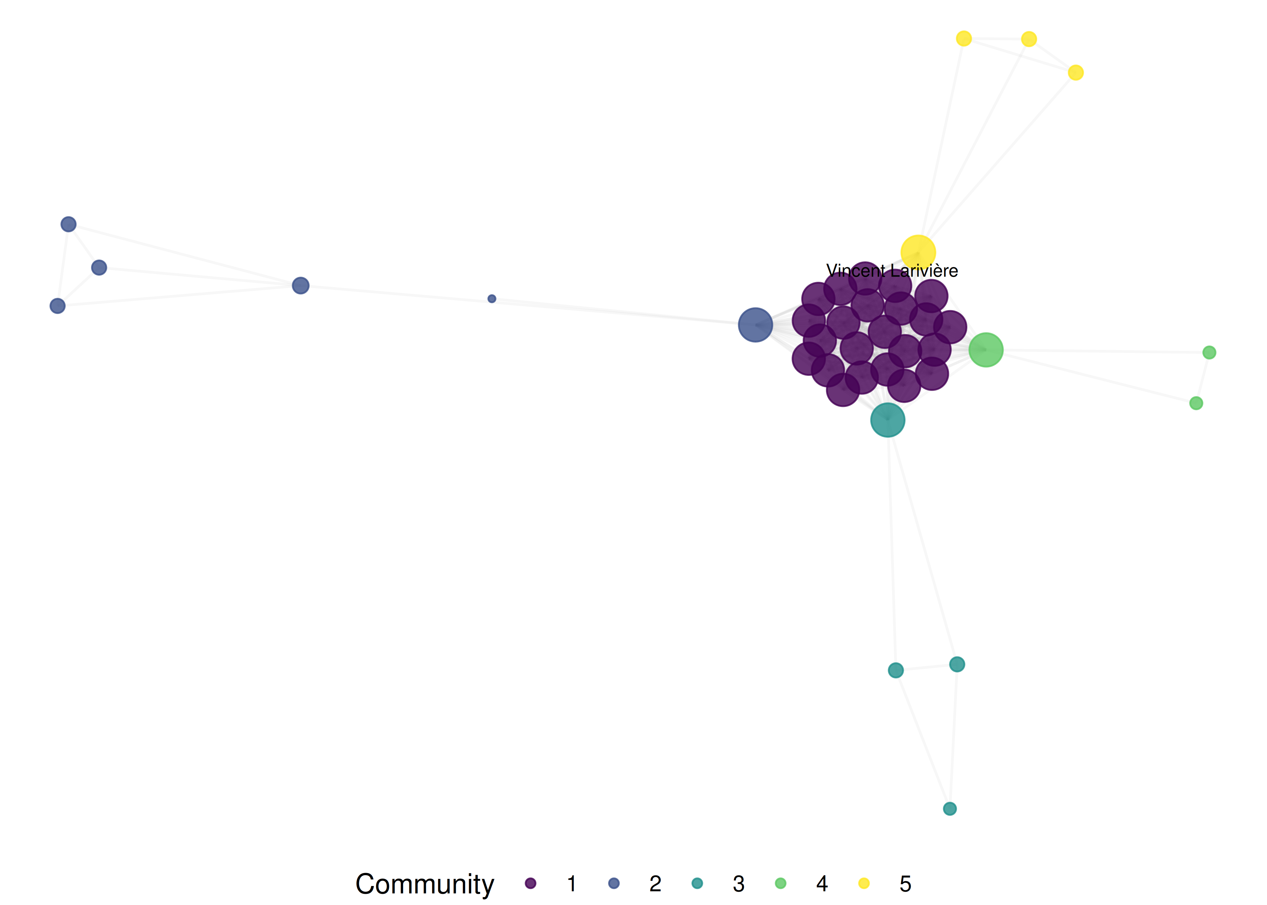
Figure 21.3: Publication-ready co-authorship network with labelled high-degree nodes.
21.5 Diagnostics and interpretation
- Layout quality: A good layout separates communities visually, minimises edge crossings, and distributes nodes evenly. If communities overlap heavily, try a different algorithm or increase the number of layout iterations.
- Readability: If the network is too dense to read, reduce the number of nodes (filter by degree), increase edge transparency, or remove edges below a weight threshold.
-
Colour distinguishability: Test figures in greyscale and with colour-blindness simulators. Viridis-based palettes (used by
palette_sci()) are designed for this. - Export verification: After exporting, open the file in the target tool (Gephi, VOSviewer) to verify that node attributes, edge weights, and labels transferred correctly.
21.7 Limitations and responsible use
- Visualisation is not analysis. A network figure is a communication tool. The visual impression can mislead if the layout, filtering, or colour encoding obscures structure. Always report the quantitative metrics alongside figures.
- Layout is not geography. Absolute positions in a force-directed layout are meaningless; only relative distances carry information. Never compare positions across different layouts or runs without the same seed.
- Large networks are unreadable. Beyond ~500 nodes, static network plots become unintelligible. Use interactive visualisation, backbone extraction (19.4), or subnetwork extraction for large data.
- Export formats lose information. GraphML preserves most attributes; Pajek format is more limited. Always verify exports and document what was lost (Hicks et al. 2015).
21.9 Common pitfalls
-
Forgetting
set.seed(). Without a fixed seed, force-directed layouts change every render, making figures irreproducible across HTML and PDF. - Encoding too many variables. Mapping degree to size, community to colour, and betweenness to transparency creates visual overload. Choose two visual channels at most.
-
Using default igraph plots. Base R
plot.igraph()produces low-quality figures. Useggraphfor publication andvisNetworkfor interactive exploration. - Exporting without coordinates. If you export a network to Gephi without coordinates, Gephi will recompute the layout, producing a different figure than your R output.
21.10 Exercises
Layout comparison. Apply five different layout algorithms to the same network. Which layout best reveals the community structure? Time each layout and report the trade-off between quality and speed.
Interactive filtering. Create a
visNetworkvisualisation where users can filter by community membership. Add a dropdown selector for community.Gephi round-trip. Export the network to GraphML, import into Gephi, apply a Force Atlas 2 layout, export as PDF. Compare the Gephi figure with the ggraph version.
Colour-blind check. Render the network figure with 3, 5, and 10 communities. At what point do the viridis colours become hard to distinguish? Test with a colour-blindness simulator.
21.11 Solutions
Solutions are provided in 2.11.
21.12 Further reading
- Bastian et al. (2009) — Gephi: an open-source platform for network visualisation and exploration.
- Fortunato (2010) — Community detection methods with extensive visualisation examples.
- Waltman et al. (2010) — VOSviewer’s approach to bibliometric network visualisation.
-
Aria and Cuccurullo (2017) —
bibliometrixincludes network visualisation viabiblioshiny().
21.13 Session info
#> R version 4.4.1 (2024-06-14)
#> Platform: x86_64-pc-linux-gnu
#> Running under: Ubuntu 24.04.4 LTS
#>
#> Matrix products: default
#> BLAS:   /usr/lib/x86_64-linux-gnu/openblas-pthread/libblas.so.3
#> LAPACK: /usr/lib/x86_64-linux-gnu/openblas-pthread/libopenblasp-r0.3.26.so;  LAPACK version 3.12.0
#>
#> locale:
#>  [1] LC_CTYPE=C.UTF-8       LC_NUMERIC=C           LC_TIME=C.UTF-8
#>  [4] LC_COLLATE=C.UTF-8     LC_MONETARY=C.UTF-8    LC_MESSAGES=C.UTF-8
#>  [7] LC_PAPER=C.UTF-8       LC_NAME=C              LC_ADDRESS=C
#> [10] LC_TELEPHONE=C         LC_MEASUREMENT=C.UTF-8 LC_IDENTIFICATION=C
#>
#> time zone: UTC
#> tzcode source: system (glibc)
#>
#> attached base packages:
#> [1] stats     graphics  grDevices utils     datasets  methods   base
#>
#> other attached packages:
#>  [1] visNetwork_2.1.4   ggraph_2.2.2       tidygraph_1.3.1    igraph_2.3.2
#>  [5] quanteda_4.4       pdftools_3.9.0     arrow_24.0.0       bibliometrix_5.4.0
#>  [9] RefManageR_1.4.0   bib2df_1.1.2.0     rcrossref_1.2.1    gt_1.3.0
#> [13] tidytext_0.4.3     glue_1.8.1         openalexR_3.0.1    lubridate_1.9.5
#> [17] forcats_1.0.1      stringr_1.6.0      dplyr_1.2.1        purrr_1.2.2
#> [21] readr_2.2.0        tidyr_1.3.2        tibble_3.3.1       ggplot2_4.0.3
#> [25] tidyverse_2.0.0
#>
#> loaded via a namespace (and not attached):
#>   [1] bibtex_0.5.2           RColorBrewer_1.1-3     rstudioapi_0.18.0
#>   [4] jsonlite_2.0.0         magrittr_2.0.5         farver_2.1.2
#>   [7] rmarkdown_2.31         fs_2.1.0               vctrs_0.7.3
#>  [10] memoise_2.0.1          askpass_1.2.1          base64enc_0.1-6
#>  [13] htmltools_0.5.9        contentanalysis_1.0.0  curl_7.1.0
#>  [16] janeaustenr_1.0.0      cellranger_1.1.0       sass_0.4.10
#>  [19] bslib_0.11.0           htmlwidgets_1.6.4      tokenizers_0.3.0
#>  [22] plyr_1.8.9             httr2_1.2.2            plotly_4.12.0
#>  [25] cachem_1.1.0           dimensionsR_0.0.3      mime_0.13
#>  [28] lifecycle_1.0.5        pkgconfig_2.0.3        Matrix_1.7-0
#>  [31] R6_2.6.1               fastmap_1.2.0          shiny_1.13.0
#>  [34] digest_0.6.39          patchwork_1.3.2        shinycssloaders_1.1.0
#>  [37] rprojroot_2.1.1        SnowballC_0.7.1        labeling_0.4.3
#>  [40] urltools_1.7.3.1       timechange_0.4.0       polyclip_1.10-7
#>  [43] httr_1.4.8             compiler_4.4.1         here_1.0.2
#>  [46] bit64_4.8.0            withr_3.0.2            S7_0.2.2
#>  [49] backports_1.5.1        viridis_0.6.5          ggforce_0.5.0
#>  [52] MASS_7.3-60.2          rappdirs_0.3.4         bibliometrixData_0.3.0
#>  [55] tools_4.4.1            otel_0.2.0             stopwords_2.3
#>  [58] zip_2.3.3              httpuv_1.6.17          rentrez_1.2.4
#>  [61] promises_1.5.0         grid_4.4.1             stringdist_0.9.17
#>  [64] generics_0.1.4         gtable_0.3.6           tzdb_0.5.0
#>  [67] rscopus_0.9.0          ca_0.71.1              data.table_1.18.4
#>  [70] hms_1.1.4              xml2_1.5.2             utf8_1.2.6
#>  [73] ggrepel_0.9.8          pillar_1.11.1          vroom_1.7.1
#>  [76] later_1.4.8            tweenr_2.0.3           brand.yml_0.1.0
#>  [79] lattice_0.22-6         bit_4.6.0              tidyselect_1.2.1
#>  [82] miniUI_0.1.2           downlit_0.4.5          knitr_1.51
#>  [85] gridExtra_2.3          bookdown_0.46          crul_1.6.0
#>  [88] xfun_0.57              graphlayouts_1.2.3     DT_0.34.0
#>  [91] humaniformat_0.6.0     stringi_1.8.7          lazyeval_0.2.3
#>  [94] qpdf_1.4.1             yaml_2.3.12            evaluate_1.0.5
#>  [97] codetools_0.2-20       httpcode_0.3.0         cli_3.6.6
#> [100] xtable_1.8-8           jquerylib_0.1.4        dichromat_2.0-0.1
#> [103] Rcpp_1.1.1-1.1         readxl_1.4.5           triebeard_0.4.1
#> [106] XML_3.99-0.23          parallel_4.4.1         assertthat_0.2.1
#> [109] pubmedR_1.0.2          viridisLite_0.4.3      scales_1.4.0
#> [112] crayon_1.5.3           openxlsx_4.2.8.1       rlang_1.2.0
#> [115] fastmatch_1.1-8