14 Institutional and Country Analysis
14.1 Learning objectives
After completing this chapter, you will be able to:
- Aggregate bibliometric data at institutional and country levels using OpenAlex
- Explain the difference between full counting and fractional counting and when each is appropriate
- Use ROR (Research Organization Registry) identifiers for reliable institutional matching
- Compute size-independent indicators (MNCS, PP(top 10%)) at the institutional level
- Interpret institutional rankings critically, accounting for size, field mix, and counting method
14.3 Conceptual background
Comparing research performance across institutions and countries is one of the most common — and most contentious — applications of bibliometrics. University rankings, national R&D assessments, and funding allocation decisions all rely on aggregate bibliometric statistics. Getting the aggregation right matters enormously.
The fundamental choice is between full counting and fractional counting. Under full counting, each institution listed on a paper receives one full credit for that paper. A paper with authors from five institutions thus generates five institutional publications. Under fractional counting, credit is divided: each institution receives 1/5 of a publication count. Full counting inflates the output of institutions that frequently collaborate, while fractional counting better reflects each entity’s proportional contribution (Glänzel and Schubert 2004; Waltman et al. 2011).
ROR (Research Organization Registry) identifiers provide a stable, open system for identifying institutions, analogous to DOIs for publications and ORCID for researchers. OpenAlex maps institutional affiliations to ROR IDs, though coverage varies by discipline and geography. Using ROR avoids the pitfalls of string matching on institution names, which are notoriously inconsistent (e.g., “MIT”, “Massachusetts Institute of Technology”, “Mass. Inst. Tech.”).
Size-independent indicators are essential for fair comparison. Raw publication counts favour large universities. The Mean Normalised Citation Score (MNCS) (Waltman et al. 2011) and PP(top 10%) — the proportion of papers in the top 10% most cited in their field and year — allow meaningful comparison between a small specialised institute and a large comprehensive university. The Leiden Ranking uses these indicators with fractional counting as its default, offering a model of responsible institutional benchmarking.
Country-level analysis faces the same choices. Additionally, linguistic bias in databases means that countries where English is not the primary research language may appear less productive than they truly are (Visser et al. 2021).
14.4 Worked example
14.4.1 Selecting institutions
We compare five research-intensive universities.
institutions <- tribble(
  ~short_name,  ~ror_id,
  "MIT",        "I63966007",
  "Oxford",     "I40120149",
  "ETH Zurich", "I202697423",
  "U Tokyo",    "I39804265",
  "U Cape Town", "I173603587"
)
14.4.2 Fetching institutional publications
fetch_inst_works <- function(inst_id) {
  res <- tryCatch(
    oa_fetch(
      entity = "works",
      authorships.institutions.id = inst_id,
      from_publication_date = "2020-01-01",
      to_publication_date = "2022-12-31",
      type = "article",
      options = list(sample = 400, seed = 42)
    ),
    error = function(e) NULL
  )
  if (is.null(res)) tibble() else res
}

inst_data <- institutions |>
  mutate(works = map(ror_id, fetch_inst_works)) |>
  filter(map_int(works, nrow) > 0)
14.4.3 Full counting vs. fractional counting
compute_counts <- function(works_df, inst_id) {
  if (is.null(works_df) || nrow(works_df) == 0) {
    return(tibble(full_count = 0L, frac_count = 0))
  }
  # Full count: each paper counts as 1
  full_count <- nrow(works_df)

  # Fractional count: 1 / number of distinct institutions per paper
  frac <- works_df |>
    select(id, authorships) |>
    unnest(authorships, names_sep = "_") |>
    unnest(authorships_affiliations, names_sep = "_") |>
    group_by(id) |>
    summarise(n_inst = n_distinct(authorships_affiliations_id), .groups = "drop") |>
    mutate(frac_credit = 1 / pmax(n_inst, 1))

  frac_count <- sum(frac$frac_credit)

  tibble(full_count = full_count, frac_count = round(frac_count, 1))
}

counting_comparison <- inst_data |>
  mutate(counts = map2(works, ror_id, compute_counts)) |>
  unnest(counts) |>
  select(short_name, full_count, frac_count) |>
  mutate(ratio = round(frac_count / full_count, 2))

counting_comparison |>
  gt() |>
  cols_label(
    short_name = "Institution",
    full_count = "Full count",
    frac_count = "Fractional count",
    ratio = "Frac / Full"
)| Institution | Full count | Fractional count | Frac / Full |
|---|---|---|---|
| MIT | 400 | 161 | 0.40 |
| Oxford | 400 | 139 | 0.35 |
| ETH Zurich | 400 | 146 | 0.37 |
14.4.4 Normalised citation impact
inst_impact <- inst_data |>
  mutate(
    mean_cites = map_dbl(works, \(w) mean(w$cited_by_count, na.rm = TRUE)),
    median_cites = map_dbl(works, \(w) median(w$cited_by_count, na.rm = TRUE)),
    mncs_approx = map_dbl(works, \(w) {
      w |>
        mutate(year = year(publication_date)) |>
        group_by(year) |>
        mutate(field_mean = mean(cited_by_count)) |>
        ungroup() |>
        mutate(ncs = cited_by_count / pmax(field_mean, 0.01)) |>
        pull(ncs) |>
        mean(na.rm = TRUE)
    })
  ) |>
  select(short_name, mean_cites, median_cites, mncs_approx) |>
  arrange(desc(mncs_approx))

inst_impact |>
  gt() |>
fmt_number(columns = c(mean_cites, mncs_approx), decimals = 2)| short_name | mean_cites | median_cites | mncs_approx |
|---|---|---|---|
| MIT | 36.22 | 13 | 1.00 |
| Oxford | 37.90 | 14 | 1.00 |
| ETH Zurich | 31.26 | 13 | 1.00 |
14.4.5 Visualization
counting_long <- counting_comparison |>
  pivot_longer(cols = c(full_count, frac_count),
               names_to = "method", values_to = "count") |>
  mutate(method = recode(method,
                         full_count = "Full counting",
                         frac_count = "Fractional counting"))

ggplot(counting_long, aes(x = count, y = reorder(short_name, count),
                          fill = method)) +
  geom_col(position = "dodge", width = 0.7) +
  scale_fill_manual(values = palette_sci(2)) +
  labs(x = "Publication count", y = NULL, fill = "Method") +
  theme_sci()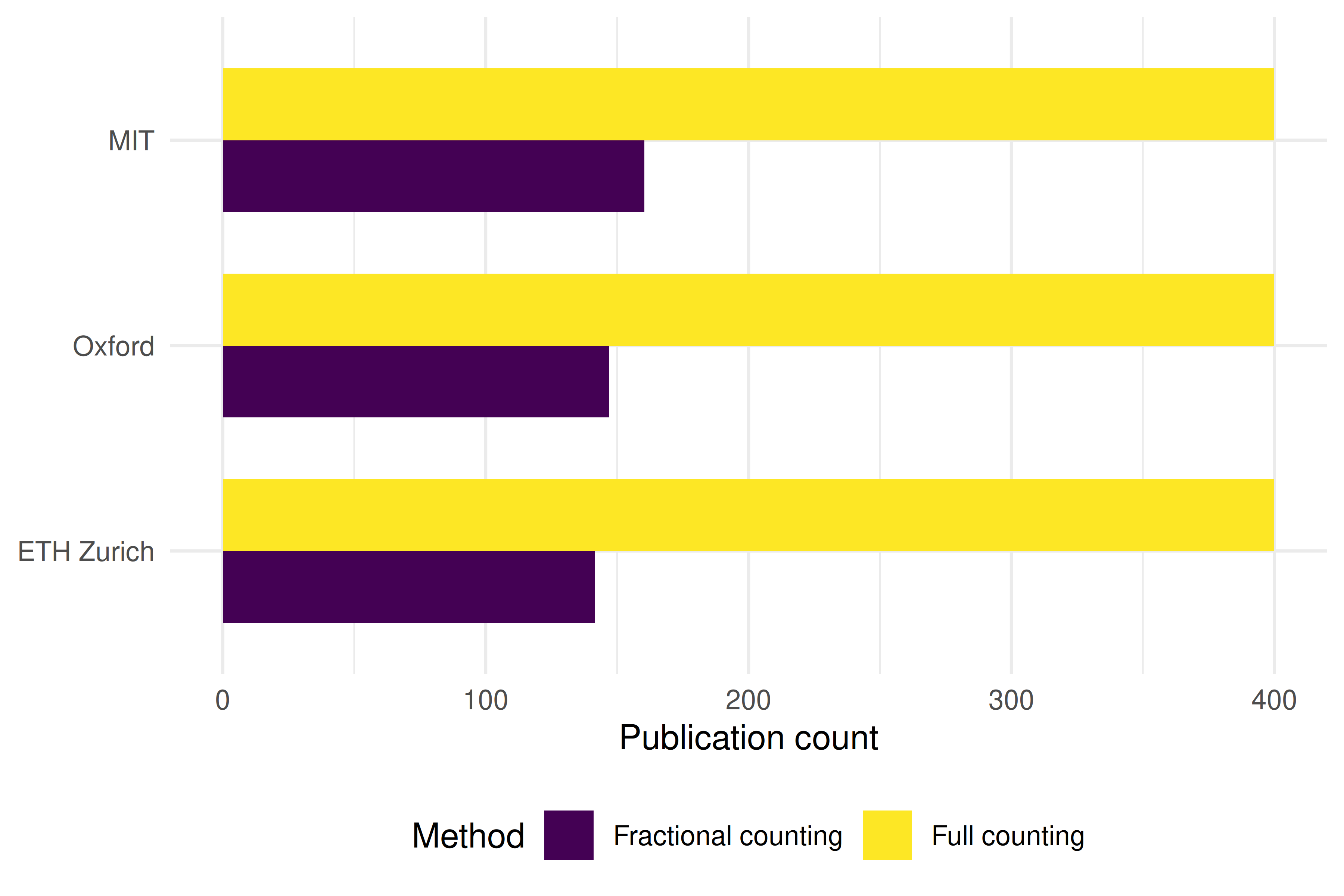
Figure 14.1: Full count vs. fractional count publication output for five institutions.
ggplot(inst_impact, aes(x = mncs_approx, y = reorder(short_name, mncs_approx))) +
  geom_col(fill = palette_sci(1)) +
  geom_vline(xintercept = 1, linetype = "dashed", colour = "grey50") +
  labs(x = "MNCS (approx.)", y = NULL) +
  theme_sci()
Figure 14.2: Approximate MNCS for each institution (within-sample normalisation).
14.5 Diagnostics and interpretation
- Size vs. impact: A large university may rank highly on total output but poorly on per-paper impact. Always report both size-dependent and size-independent indicators.
- Field mix: A medical university will appear more productive (and highly cited) than a social-science institute due to field-level citation norms. True normalisation requires field-level data.
- Sample vs. population: Our sample of 400 works per institution is illustrative. For real benchmarking, use the full population or report confidence intervals.
- Fractional/full ratio: A ratio near 1.0 indicates few collaborations beyond the institution; a ratio well below 1.0 indicates extensive inter-institutional collaboration.
14.7 Limitations and responsible use
- Rankings oversimplify. Institutional and country rankings compress a multidimensional reality into a single number. The Leiden Manifesto (Hicks et al. 2015) warns against using rankings mechanically.
- Affiliation data quality. Not all papers have complete or correct institutional affiliations. OpenAlex coverage depends on publisher metadata quality.
- Counting method changes conclusions. The same data can yield different institutional rankings depending on whether full or fractional counting is used. Always report the method.
- Language and geographic bias. Databases undercount research published in non-English languages, disadvantaging countries in Latin America, Asia, and Africa (Visser et al. 2021; Singh et al. 2021).
- Do not compare across fields without normalisation. A biomedical research university will always outperform a humanities-focused institution on raw citation indicators.
14.9 Common pitfalls
- Using full counting when fractional is more appropriate. Full counting double-credits collaborative work, inflating output for institutions with many international partnerships.
- Ignoring field normalisation. Comparing raw MNCS across institutions with very different disciplinary profiles is misleading.
- String-matching institution names. Never match institutions by name strings alone. Use ROR or OpenAlex institution IDs.
- Treating samples as populations. If you sampled 400 works per institution, the resulting metrics have uncertainty. Report this.
- Forgetting subsidiary institutions. Large universities may have hospitals, research institutes, or campuses with separate ROR IDs. Decide on the unit of analysis upfront.
14.10 Exercises
Country-level analysis. Aggregate publications by author country (using
authorships.countries) instead of institution. Compute full and fractional counts for the top 10 countries in your corpus. Which countries are most affected by the counting method?PP(top 10%) by institution. For each institution, compute the proportion of papers in the top 10% most cited within the sample (by year). How does this correlate with MNCS?
Collaboration intensity. Compute the mean number of distinct institutional affiliations per paper for each institution. Is there a relationship between collaboration intensity and the full/fractional count ratio?
14.11 Solutions
Solutions are provided in 2.11.
14.12 Further reading
- Waltman et al. (2011) — MNCS and size-independent indicators for institutional comparison.
- Glänzel and Schubert (2004) — Fractional counting in co-authorship and institutional analysis.
- Hicks et al. (2015) — The Leiden Manifesto on responsible institutional benchmarking.
- Waltman (2016) — Review of citation impact indicators applicable to institutions and countries.
- Visser et al. (2021) — Database coverage comparison; crucial context for country-level analysis.
- Singh et al. (2021) — Journal coverage across databases, highlighting geographic imbalances.
14.13 Session info
#> R version 4.4.1 (2024-06-14)
#> Platform: x86_64-pc-linux-gnu
#> Running under: Ubuntu 24.04.4 LTS
#>
#> Matrix products: default
#> BLAS:   /usr/lib/x86_64-linux-gnu/openblas-pthread/libblas.so.3
#> LAPACK: /usr/lib/x86_64-linux-gnu/openblas-pthread/libopenblasp-r0.3.26.so;  LAPACK version 3.12.0
#>
#> locale:
#>  [1] LC_CTYPE=C.UTF-8       LC_NUMERIC=C           LC_TIME=C.UTF-8
#>  [4] LC_COLLATE=C.UTF-8     LC_MONETARY=C.UTF-8    LC_MESSAGES=C.UTF-8
#>  [7] LC_PAPER=C.UTF-8       LC_NAME=C              LC_ADDRESS=C
#> [10] LC_TELEPHONE=C         LC_MEASUREMENT=C.UTF-8 LC_IDENTIFICATION=C
#>
#> time zone: UTC
#> tzcode source: system (glibc)
#>
#> attached base packages:
#> [1] stats     graphics  grDevices utils     datasets  methods   base
#>
#> other attached packages:
#>  [1] quanteda_4.4       pdftools_3.9.0     arrow_24.0.0       bibliometrix_5.4.0
#>  [5] RefManageR_1.4.0   bib2df_1.1.2.0     rcrossref_1.2.1    gt_1.3.0
#>  [9] tidytext_0.4.3     glue_1.8.1         openalexR_3.0.1    lubridate_1.9.5
#> [13] forcats_1.0.1      stringr_1.6.0      dplyr_1.2.1        purrr_1.2.2
#> [17] readr_2.2.0        tidyr_1.3.2        tibble_3.3.1       ggplot2_4.0.3
#> [21] tidyverse_2.0.0
#>
#> loaded via a namespace (and not attached):
#>   [1] bibtex_0.5.2           RColorBrewer_1.1-3     rstudioapi_0.18.0
#>   [4] jsonlite_2.0.0         magrittr_2.0.5         farver_2.1.2
#>   [7] rmarkdown_2.31         fs_2.1.0               vctrs_0.7.3
#>  [10] memoise_2.0.1          askpass_1.2.1          base64enc_0.1-6
#>  [13] htmltools_0.5.9        contentanalysis_1.0.0  curl_7.1.0
#>  [16] janeaustenr_1.0.0      cellranger_1.1.0       sass_0.4.10
#>  [19] bslib_0.11.0           htmlwidgets_1.6.4      tokenizers_0.3.0
#>  [22] plyr_1.8.9             httr2_1.2.2            plotly_4.12.0
#>  [25] cachem_1.1.0           dimensionsR_0.0.3      igraph_2.3.2
#>  [28] mime_0.13              lifecycle_1.0.5        pkgconfig_2.0.3
#>  [31] Matrix_1.7-0           R6_2.6.1               fastmap_1.2.0
#>  [34] shiny_1.13.0           digest_0.6.39          shinycssloaders_1.1.0
#>  [37] rprojroot_2.1.1        SnowballC_0.7.1        labeling_0.4.3
#>  [40] urltools_1.7.3.1       timechange_0.4.0       httr_1.4.8
#>  [43] compiler_4.4.1         here_1.0.2             bit64_4.8.0
#>  [46] withr_3.0.2            S7_0.2.2               backports_1.5.1
#>  [49] viridis_0.6.5          rappdirs_0.3.4         bibliometrixData_0.3.0
#>  [52] tools_4.4.1            otel_0.2.0             stopwords_2.3
#>  [55] zip_2.3.3              httpuv_1.6.17          rentrez_1.2.4
#>  [58] promises_1.5.0         grid_4.4.1             stringdist_0.9.17
#>  [61] generics_0.1.4         gtable_0.3.6           tzdb_0.5.0
#>  [64] rscopus_0.9.0          ca_0.71.1              data.table_1.18.4
#>  [67] hms_1.1.4              xml2_1.5.2             utf8_1.2.6
#>  [70] ggrepel_0.9.8          pillar_1.11.1          later_1.4.8
#>  [73] brand.yml_0.1.0        lattice_0.22-6         bit_4.6.0
#>  [76] tidyselect_1.2.1       miniUI_0.1.2           downlit_0.4.5
#>  [79] knitr_1.51             gridExtra_2.3          bookdown_0.46
#>  [82] crul_1.6.0             xfun_0.57              DT_0.34.0
#>  [85] humaniformat_0.6.0     visNetwork_2.1.4       stringi_1.8.7
#>  [88] lazyeval_0.2.3         qpdf_1.4.1             yaml_2.3.12
#>  [91] evaluate_1.0.5         codetools_0.2-20       httpcode_0.3.0
#>  [94] cli_3.6.6              xtable_1.8-8           jquerylib_0.1.4
#>  [97] dichromat_2.0-0.1      Rcpp_1.1.1-1.1         readxl_1.4.5
#> [100] triebeard_0.4.1        XML_3.99-0.23          parallel_4.4.1
#> [103] assertthat_0.2.1       pubmedR_1.0.2          viridisLite_0.4.3
#> [106] scales_1.4.0           openxlsx_4.2.8.1       rlang_1.2.0
#> [109] fastmatch_1.1-8