37 Parameterized Quarto Reports
37.1 Learning objectives
After completing this chapter, you will be able to:
- Define parameters in a Quarto document’s YAML header
- Access parameters in R code chunks to drive data retrieval and analysis
- Render parameterized reports from the command line and from scripts
- Build a template for journal-level bibliometric profiles
- Generate multiple reports in batch using purrr or shell loops
37.3 Conceptual background
Many bibliometric tasks are repetitive: generating the same analysis for 10 journals, 5 departments, or 20 funders. Writing separate scripts for each entity is error-prone and hard to maintain. Parameterized reports solve this by defining variables (parameters) that change the report’s content without changing its structure.
Quarto supports parameters via the params field in the YAML header. Parameters can be strings, numbers, or lists. Inside the document, params$journal_id (or params$institution) drives data fetching, filtering, and labelling. At render time, parameter values are passed via the command line or a rendering script.
This approach scales naturally: a loop or purrr::walk() call renders dozens of reports with different parameters, producing a complete portfolio of bibliometric profiles with consistent methodology and formatting.
Parameterized reports are especially valuable for institutional reporting (annual bibliometric profiles for each department), journal analytics (quarterly reports for a publisher’s journal portfolio), and funding assessment (per-grant output summaries).
37.4 Worked example
37.4.1 Defining parameters
A parameterized Quarto document starts with parameters in the YAML header:
# Example YAML header (not executable R):
#
# ---
# title: "Journal Bibliometric Profile"
# params:
#   journal_id: "S148561398"
#   journal_name: "Scientometrics"
#   start_year: 2020
#   end_year: 2023
# ---
37.4.2 Using parameters in code
journal_id <- "S148561398"
journal_name <- "Scientometrics"
start_year <- 2020
end_year <- 2023
works <- oa_fetch(
  entity = "works",
  primary_location.source.id = journal_id,
  from_publication_date = paste0(start_year, "-01-01"),
  to_publication_date = paste0(end_year, "-12-31"),
  type = "article",
  options = list(sample = 300, seed = 42)
)

cat(glue("Journal: {journal_name}\n"))
#> Journal: Scientometrics#> Period: 2020--2023#> Articles retrieved: 30037.4.3 Automated summary statistics
summary_stats <- works |>
  summarise(
    total_articles = n(),
    mean_citations = round(mean(cited_by_count), 1),
    median_citations = median(cited_by_count),
    h_index = compute_h_index(cited_by_count),
    oa_rate = round(mean(oa_status != "closed", na.rm = TRUE) * 100, 1)
  ) |>
  mutate(across(everything(), as.character)) |>
  pivot_longer(everything(), names_to = "Metric", values_to = "Value")

summary_stats |> gt()| Metric | Value |
|---|---|
| total_articles | 300 |
| mean_citations | 18.6 |
| median_citations | 12 |
| h_index | 37 |
| oa_rate | 48 |
37.4.4 Parameterized figure
works |>
  mutate(year = year(publication_date)) |>
  count(year) |>
  ggplot(aes(x = factor(year), y = n)) +
  geom_col(fill = palette_sci(1)) +
  labs(x = "Year", y = "Articles",
       title = glue("{journal_name} — Annual Output")) +
  theme_sci()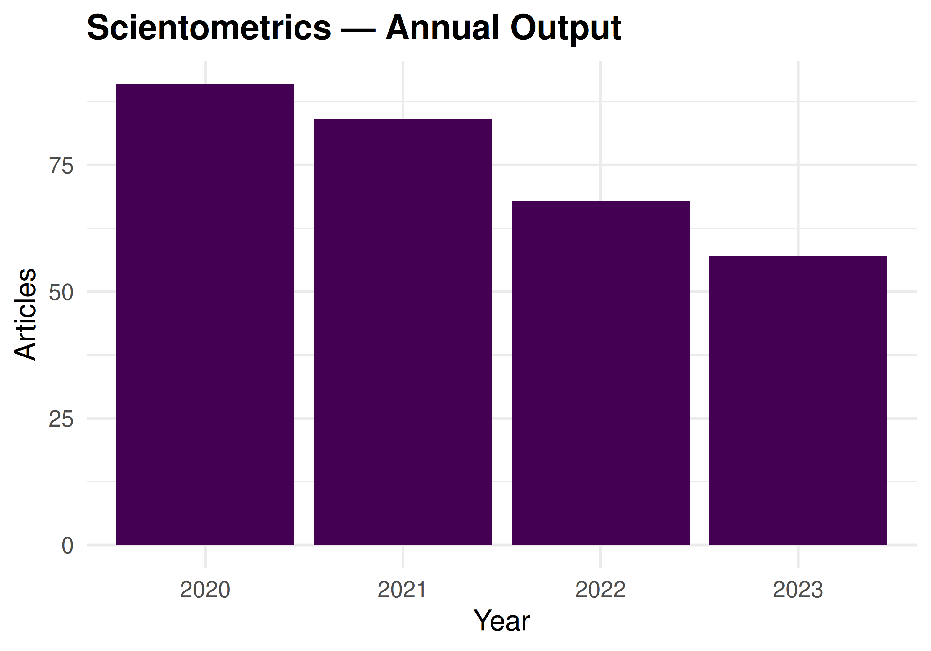
Figure 37.1: Annual publication count for the selected journal.
37.4.5 Batch rendering
# Render for multiple journals:
journals <- tibble(
  journal_id = c("S148561398", "S202381698", "S137773608"),
  journal_name = c("Scientometrics", "PLOS ONE", "Nature")
)

walk2(journals$journal_id, journals$journal_name, function(jid, jname) {
  quarto::quarto_render(
    input = "journal_profile.qmd",
    execute_params = list(
      journal_id = jid,
      journal_name = jname,
      start_year = 2020,
      end_year = 2023
    ),
    output_file = glue("reports/{jname}_profile.html")
  )
})
37.5 Diagnostics and interpretation
- Parameter validation: Check that parameters produce valid API queries. Invalid journal IDs return empty results silently.
-
Sample consistency: When using
options = list(sample = N), the sample changes if the underlying corpus changes. Useseedfor stability. - Output naming: Automated file naming should avoid special characters. Sanitise journal names before using them in file paths.
- Error handling: Batch rendering should catch and log errors for individual reports without stopping the entire batch.
37.7 Limitations and responsible use
- Automated ≠ mindless. Parameterized reports produce consistent output but still require human review. An automated report with a data error will produce the wrong results consistently across all entities.
- One template fits all? Different entities may need different analyses. A template designed for a large journal may produce misleading results for a small one (e.g., sparse yearly bins).
- API costs. Batch rendering for 100 journals makes 100 API calls. Respect rate limits and cache results.
- Report fatigue. Generating too many reports can overwhelm decision-makers. Produce reports for entities that need them, not for every possible parameter value (Hicks et al. 2015).
37.9 Common pitfalls
- Hardcoding values that should be parameters. If you find yourself editing a date or ID in the script, it should be a parameter.
- Not testing with extreme parameters. A journal with 5 papers per year needs different visualisations than one with 5,000. Test edge cases.
-
Rendering without caching. Each render re-executes all code. Use Quarto’s
cache: trueor file-based caching to avoid redundant API calls. - Forgetting output format compatibility. Interactive widgets work in HTML but not PDF. Ensure your template degrades gracefully.
37.10 Exercises
Institutional template. Create a parameterized Quarto document for institutional profiles. Parameters: institution ID, name, start year, end year. Include publication count, citation distribution, and top authors.
Batch rendering. Render the journal profile template for 3 different journals. Compare the resulting reports side by side.
Conditional content. Add conditional logic: if the sample has fewer than 50 papers, display a warning message instead of the citation distribution figure.
37.11 Solutions
Solutions are provided in 2.11.
37.13 Session info
#> R version 4.4.1 (2024-06-14)
#> Platform: x86_64-pc-linux-gnu
#> Running under: Ubuntu 24.04.4 LTS
#>
#> Matrix products: default
#> BLAS:   /usr/lib/x86_64-linux-gnu/openblas-pthread/libblas.so.3
#> LAPACK: /usr/lib/x86_64-linux-gnu/openblas-pthread/libopenblasp-r0.3.26.so;  LAPACK version 3.12.0
#>
#> locale:
#>  [1] LC_CTYPE=C.UTF-8       LC_NUMERIC=C           LC_TIME=C.UTF-8
#>  [4] LC_COLLATE=C.UTF-8     LC_MONETARY=C.UTF-8    LC_MESSAGES=C.UTF-8
#>  [7] LC_PAPER=C.UTF-8       LC_NAME=C              LC_ADDRESS=C
#> [10] LC_TELEPHONE=C         LC_MEASUREMENT=C.UTF-8 LC_IDENTIFICATION=C
#>
#> time zone: UTC
#> tzcode source: system (glibc)
#>
#> attached base packages:
#> [1] stats     graphics  grDevices utils     datasets  methods   base
#>
#> other attached packages:
#>  [1] DT_0.34.0                 plotly_4.12.0
#>  [3] uwot_0.2.4                Matrix_1.7-0
#>  [5] word2vec_0.4.1            stm_1.3.8
#>  [7] topicmodels_0.2-17        quanteda.textstats_0.97.2
#>  [9] visNetwork_2.1.4          ggraph_2.2.2
#> [11] tidygraph_1.3.1           igraph_2.3.2
#> [13] quanteda_4.4              pdftools_3.9.0
#> [15] arrow_24.0.0              bibliometrix_5.4.0
#> [17] RefManageR_1.4.0          bib2df_1.1.2.0
#> [19] rcrossref_1.2.1           gt_1.3.0
#> [21] tidytext_0.4.3            glue_1.8.1
#> [23] openalexR_3.0.1           lubridate_1.9.5
#> [25] forcats_1.0.1             stringr_1.6.0
#> [27] dplyr_1.2.1               purrr_1.2.2
#> [29] readr_2.2.0               tidyr_1.3.2
#> [31] tibble_3.3.1              ggplot2_4.0.3
#> [33] tidyverse_2.0.0
#>
#> loaded via a namespace (and not attached):
#>   [1] splines_4.4.1          later_1.4.8            urltools_1.7.3.1
#>   [4] cellranger_1.1.0       triebeard_0.4.1        polyclip_1.10-7
#>   [7] XML_3.99-0.23          lifecycle_1.0.5        httr2_1.2.2
#>  [10] rprojroot_2.1.1        NLP_0.3-2              lattice_0.22-6
#>  [13] brand.yml_0.1.0        vroom_1.7.1            MASS_7.3-60.2
#>  [16] crosstalk_1.2.2        backports_1.5.1        SnowballC_0.7.1
#>  [19] magrittr_2.0.5         openxlsx_4.2.8.1       sass_0.4.10
#>  [22] rmarkdown_2.31         jquerylib_0.1.4        yaml_2.3.12
#>  [25] httpuv_1.6.17          otel_0.2.0             zip_2.3.3
#>  [28] askpass_1.2.1          RColorBrewer_1.1-3     downlit_0.4.5
#>  [31] contentanalysis_1.0.0  tweenr_2.0.3           rappdirs_0.3.4
#>  [34] tm_0.7-18              ggrepel_0.9.8          tokenizers_0.3.0
#>  [37] crul_1.6.0             rentrez_1.2.4          RSpectra_0.16-2
#>  [40] codetools_0.2-20       xml2_1.5.2             ggforce_0.5.0
#>  [43] tidyselect_1.2.1       rscopus_0.9.0          httpcode_0.3.0
#>  [46] farver_2.1.2           viridis_0.6.5          matrixStats_1.5.0
#>  [49] stats4_4.4.1           base64enc_0.1-6        jsonlite_2.0.0
#>  [52] tools_4.4.1            stringdist_0.9.17      Rcpp_1.1.1-1.1
#>  [55] gridExtra_2.3          xfun_0.57              here_1.0.2
#>  [58] mgcv_1.9-1             ca_0.71.1              withr_3.0.2
#>  [61] fastmap_1.2.0          digest_0.6.39          timechange_0.4.0
#>  [64] R6_2.6.1               mime_0.13              qpdf_1.4.1
#>  [67] dichromat_2.0-0.1      utf8_1.2.6             generics_0.1.4
#>  [70] data.table_1.18.4      FNN_1.1.4.1            graphlayouts_1.2.3
#>  [73] stopwords_2.3          httr_1.4.8             htmlwidgets_1.6.4
#>  [76] pkgconfig_2.0.3        gtable_0.3.6           modeltools_0.2-24
#>  [79] S7_0.2.2               janeaustenr_1.0.0      htmltools_0.5.9
#>  [82] bookdown_0.46          scales_1.4.0           knitr_1.51
#>  [85] rstudioapi_0.18.0      tzdb_0.5.0             reshape2_1.4.5
#>  [88] nlme_3.1-164           curl_7.1.0             cachem_1.1.0
#>  [91] parallel_4.4.1         miniUI_0.1.2           shinycssloaders_1.1.0
#>  [94] pubmedR_1.0.2          pillar_1.11.1          grid_4.4.1
#>  [97] vctrs_0.7.3            slam_0.1-55            promises_1.5.0
#> [100] xtable_1.8-8           evaluate_1.0.5         cli_3.6.6
#> [103] compiler_4.4.1         rlang_1.2.0            crayon_1.5.3
#> [106] labeling_0.4.3         dimensionsR_0.0.3      plyr_1.8.9
#> [109] fs_2.1.0               stringi_1.8.7          viridisLite_0.4.3
#> [112] assertthat_0.2.1       lazyeval_0.2.3         bibliometrixData_0.3.0
#> [115] hms_1.1.4              patchwork_1.3.2        bit64_4.8.0
#> [118] humaniformat_0.6.0     shiny_1.13.0           broom_1.0.12
#> [121] memoise_2.0.1          bslib_0.11.0           bibtex_0.5.2
#> [124] fastmatch_1.1-8        bit_4.6.0              nsyllable_1.0.1
#> [127] readxl_1.4.5