20 Science Mapping and Overlay Maps
20.1 Learning objectives
After completing this chapter, you will be able to:
- Explain the principles of science mapping and its applications
- Construct a journal-level co-citation network from OpenAlex data
- Create an overlay map that positions a research profile on a base map
- Interpret overlay maps to identify research strengths and gaps
- Discuss the limitations of global science maps for local evaluation
20.3 Conceptual background
A science map is a spatial representation of the structure of science, where proximity indicates relatedness. Just as a geographic map shows the layout of countries and continents, a science map shows the layout of disciplines, fields, and research areas. These maps are constructed from bibliometric data — typically citation links between journals or document sets — and visualised using network layouts or dimensionality reduction techniques.
The most common base maps use journal-level citation networks. Two journals are linked if papers in one frequently cite papers in the other. Community detection applied to these networks produces clusters corresponding to broad disciplines (biomedical sciences, physical sciences, social sciences, etc.). Waltman et al. (2010) developed methods for constructing such maps from large-scale citation data, and the resulting visualisations are widely used in science policy and institutional assessment.
An overlay map (Rafols et al. 2010) takes a global science map as a fixed background and plots a specific entity’s output on top. For example, a university’s publications are mapped to the journals in which they appeared; the overlay then shows which areas of the global map the university is active in, and how intensely. This technique is powerful for visualising research profiles, identifying strategic gaps, and comparing institutions or countries without reducing their activity to a single number.
The construction pipeline involves three steps: (1) build or obtain a base map of journals with coordinates and cluster assignments; (2) map the entity’s publications to journals in the base map; (3) scale node sizes proportionally and overlay on the base map.
Science maps provide intuitive, holistic overviews of research landscapes. However, they are projections of high-dimensional data into two dimensions, and like any projection, they introduce distortion. Interdisciplinary journals may appear in unexpected locations, and the layout algorithm’s random seed affects exact positions (Hicks et al. 2015).
20.4 Worked example
20.4.1 Building a journal co-citation base map
We construct a base map from citation flows between journals in a multidisciplinary sample.
works_multi <- oa_fetch(
  entity = "works",
  from_publication_date = "2022-01-01",
  to_publication_date = "2022-12-31",
  type = "article",
  options = list(sample = 500, seed = 42)
)

journal_data <- works_multi |>
  select(id, source_display_name, referenced_works) |>
  filter(!is.na(source_display_name)) |>
  unnest(referenced_works) |>
  rename(cited_id = referenced_works)

cat(glue("Citing papers with journal info: {n_distinct(journal_data$id)}\n"))
#> Citing papers with journal info: 478#> Unique source journals: 409
journal_cited <- journal_data |>
  select(citing_journal = source_display_name, cited_id)

journal_pairs <- journal_cited |>
  inner_join(journal_cited, by = "cited_id", suffix = c("_a", "_b"),
             relationship = "many-to-many") |>
  filter(citing_journal_a < citing_journal_b) |>
  count(citing_journal_a, citing_journal_b, name = "cocitation")

journal_pairs_top <- journal_pairs |>
  filter(cocitation >= 3)

g_journals <- graph_from_data_frame(
  journal_pairs_top |> select(citing_journal_a, citing_journal_b,
                               weight = cocitation),
  directed = FALSE
) |>
  simplify(edge.attr.comb = list(weight = "sum"))

cat(glue("Journal base map: {vcount(g_journals)} journals, {ecount(g_journals)} edges\n"))
#> Journal base map: 125 journals, 848 edges20.4.2 Clustering journals into disciplines
comm <- cluster_leiden(g_journals, resolution_parameter = 0.8,
                       objective_function = "modularity")
V(g_journals)$cluster <- as.factor(membership(comm))
V(g_journals)$degree <- degree(g_journals)

cluster_table <- tibble(
  journal = V(g_journals)$name,
  cluster = V(g_journals)$cluster,
  degree = V(g_journals)$degree
) |>
  group_by(cluster) |>
  summarise(n_journals = n(),
            top_journals = paste(head(journal[order(-degree)], 3),
                                 collapse = "; "),
            .groups = "drop") |>
  arrange(desc(n_journals))

cluster_table |> head(8) |> gt()| cluster | n_journals | top_journals |
|---|---|---|
| 1 | 125 | DOAJ (DOAJ: Directory of Open Access Journals); HAL (Le Centre pour la Communication Scientifique Directe); Institutional Repositories DataBase (IRDB) |
20.4.3 Visualising the base map
set.seed(42)
layout <- create_layout(as_tbl_graph(g_journals), layout = "fr")

ggraph(layout) +
  geom_edge_link(alpha = 0.05, colour = "grey70") +
  geom_node_point(aes(colour = cluster, size = degree), alpha = 0.7) +
  scale_size_continuous(range = c(1, 5), guide = "none") +
  scale_colour_manual(values = palette_sci(
    n_distinct(V(g_journals)$cluster)
  )) +
  labs(colour = "Cluster") +
  theme_void(base_family = "sans", base_size = 11) +
  theme(legend.position = "bottom")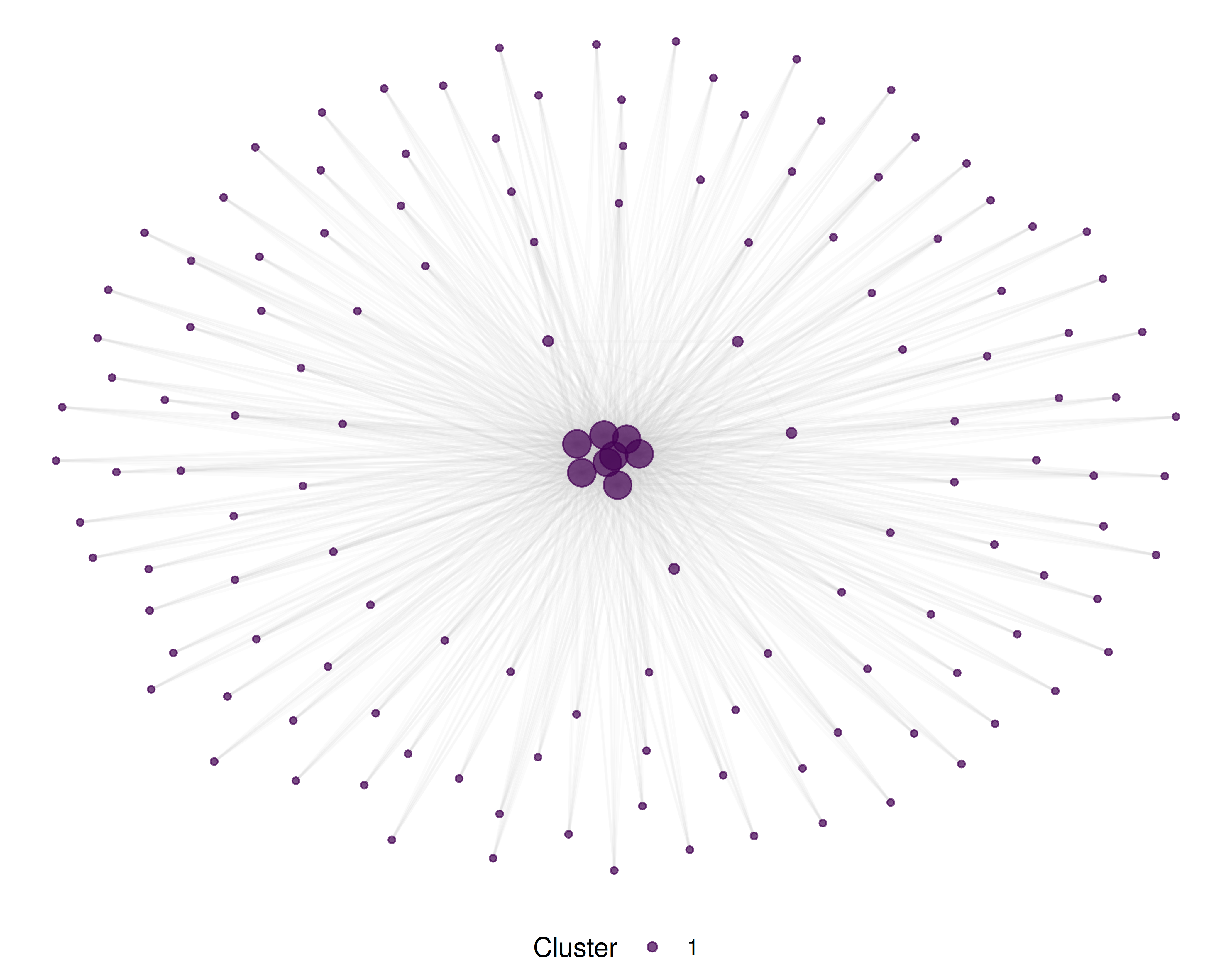
Figure 20.1: Journal co-citation base map coloured by discipline cluster.
20.4.4 Creating an overlay map
We overlay the publication profile of an institution.
inst_works <- oa_fetch(
  entity = "works",
  authorships.institutions.id = "I40120149",
  from_publication_date = "2022-01-01",
  to_publication_date = "2022-12-31",
  type = "article",
  options = list(sample = 300, seed = 42)
)

inst_journals <- inst_works |>
  filter(!is.na(source_display_name)) |>
  count(source_display_name, name = "n_pubs", sort = TRUE)

basemap_journals <- V(g_journals)$name
inst_journals_matched <- inst_journals |>
  filter(source_display_name %in% basemap_journals)

cat(glue("Institution journals matched to base map: {nrow(inst_journals_matched)} / {nrow(inst_journals)}\n"))
#> Institution journals matched to base map: 9 / 247
overlay_sizes <- tibble(journal = V(g_journals)$name) |>
  left_join(inst_journals_matched, by = c("journal" = "source_display_name")) |>
  mutate(n_pubs = replace_na(n_pubs, 0))

set.seed(42)
layout_overlay <- create_layout(as_tbl_graph(g_journals), layout = "fr")

ggraph(layout_overlay) +
  geom_edge_link(alpha = 0.03, colour = "grey80") +
  geom_node_point(colour = "grey85", size = 1.5, alpha = 0.5) +
  geom_node_point(
    data = layout_overlay |> left_join(overlay_sizes, by = c("name" = "journal")) |>
      filter(n_pubs > 0),
    aes(size = n_pubs, colour = cluster), alpha = 0.8
  ) +
  scale_size_continuous(range = c(2, 8), name = "Publications") +
  scale_colour_manual(values = palette_sci(
    n_distinct(V(g_journals)$cluster)
  )) +
  labs(colour = "Cluster") +
  theme_void(base_family = "sans", base_size = 11) +
  theme(legend.position = "bottom")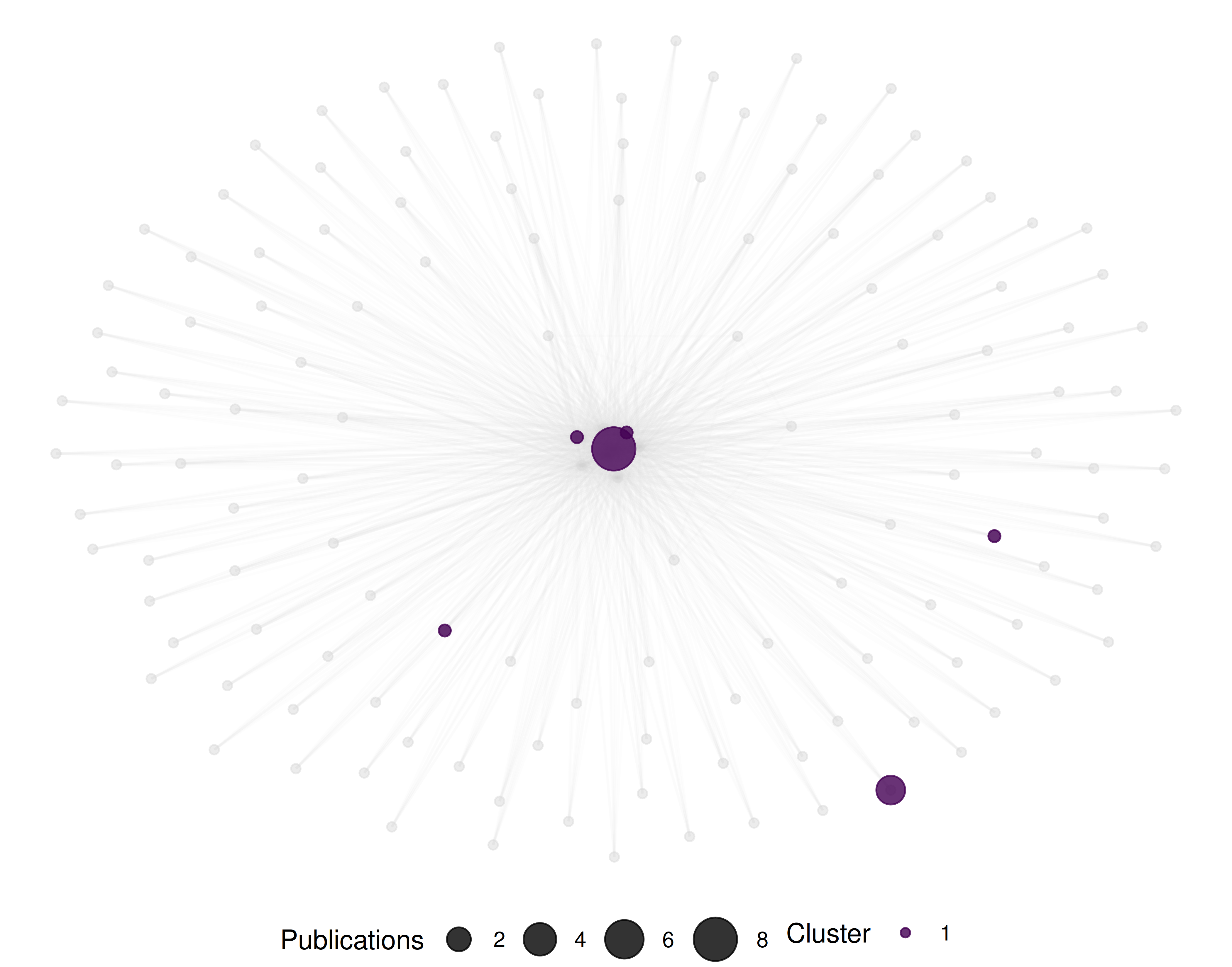
Figure 20.2: Overlay map showing Oxford’s 2022 publication profile on the journal base map.
20.5 Diagnostics and interpretation
- Journal matching rate: The fraction of the entity’s publications that match journals in the base map determines overlay completeness. Low matching rates (< 50%) indicate the base map is too narrow for the entity’s profile.
-
Layout stability: Force-directed layouts are sensitive to initial conditions. Always use
set.seed()and report the seed. Consider consensus layouts from multiple seeds for important maps. - Cluster labelling: Algorithmic clusters need human interpretation. Label clusters by inspecting the journals they contain, not by relying on the algorithm.
- Overlay concentration: If the overlay is concentrated in one or two clusters, the institution is highly specialised. Dispersed overlays indicate breadth. Neither is inherently better.
20.7 Limitations and responsible use
- Projection distortion. Two-dimensional layouts compress high-dimensional citation relationships. Journals at the boundaries between disciplines may be misplaced. Do not over-interpret exact positions.
- Journal-level aggregation. Mapping publications to journals loses within-journal variation. A paper in Nature could be biology, physics, or chemistry — the overlay cannot distinguish.
- Sample-dependent base maps. Our base map is built from a small sample. Production science maps (e.g., the CWTS journal map) use comprehensive citation data. Treat this example as illustrative.
- Not evaluative. Science maps show where research happens, not how good it is. An empty region on a university’s overlay map is not a weakness — it may reflect a deliberate strategic choice (Hicks et al. 2015).
- Interdisciplinary research is underrepresented. Journals at disciplinary boundaries may cluster with one discipline, making interdisciplinary work partially invisible (Rafols et al. 2010).
20.9 Common pitfalls
- Using too small a base map. A base map with fewer than 50 journals lacks resolution. Aim for at least 100–200 journals for meaningful discipline separation.
- Comparing overlays from different base maps. Node positions are not transferable between different base maps. To compare institutions, overlay them on the same base map.
- Ignoring unmatched publications. Publications in journals not on the base map simply disappear from the overlay. Report the matching rate.
- Treating clusters as fixed disciplines. Cluster assignments depend on the algorithm, resolution parameter, and data sample. They are analytical tools, not natural categories.
20.10 Exercises
Multi-institution overlay. Overlay the profiles of two institutions on the same base map using different colours. Where do their research profiles overlap, and where do they diverge?
Temporal overlay. Build overlays for the same institution in two different years. Has the research profile shifted toward new areas or remained stable?
Country-level overlay. Instead of an institution, overlay a country’s publication profile. How does a small specialised country (e.g., Singapore) compare to a large diversified one (e.g., the United States)?
20.11 Solutions
Solutions are provided in 2.11.
20.12 Further reading
- Rafols et al. (2010) — Overlay maps for visualising research profiles on global science maps.
- Waltman et al. (2010) — Unified approach to constructing and clustering bibliometric maps.
- Hicks et al. (2015) — The Leiden Manifesto: responsible interpretation of quantitative research profiles.
- Fortunato (2010) — Community detection methods relevant to journal clustering.
20.13 Session info
#> R version 4.4.1 (2024-06-14)
#> Platform: x86_64-pc-linux-gnu
#> Running under: Ubuntu 24.04.4 LTS
#>
#> Matrix products: default
#> BLAS:   /usr/lib/x86_64-linux-gnu/openblas-pthread/libblas.so.3
#> LAPACK: /usr/lib/x86_64-linux-gnu/openblas-pthread/libopenblasp-r0.3.26.so;  LAPACK version 3.12.0
#>
#> locale:
#>  [1] LC_CTYPE=C.UTF-8       LC_NUMERIC=C           LC_TIME=C.UTF-8
#>  [4] LC_COLLATE=C.UTF-8     LC_MONETARY=C.UTF-8    LC_MESSAGES=C.UTF-8
#>  [7] LC_PAPER=C.UTF-8       LC_NAME=C              LC_ADDRESS=C
#> [10] LC_TELEPHONE=C         LC_MEASUREMENT=C.UTF-8 LC_IDENTIFICATION=C
#>
#> time zone: UTC
#> tzcode source: system (glibc)
#>
#> attached base packages:
#> [1] stats     graphics  grDevices utils     datasets  methods   base
#>
#> other attached packages:
#>  [1] ggraph_2.2.2       tidygraph_1.3.1    igraph_2.3.2       quanteda_4.4
#>  [5] pdftools_3.9.0     arrow_24.0.0       bibliometrix_5.4.0 RefManageR_1.4.0
#>  [9] bib2df_1.1.2.0     rcrossref_1.2.1    gt_1.3.0           tidytext_0.4.3
#> [13] glue_1.8.1         openalexR_3.0.1    lubridate_1.9.5    forcats_1.0.1
#> [17] stringr_1.6.0      dplyr_1.2.1        purrr_1.2.2        readr_2.2.0
#> [21] tidyr_1.3.2        tibble_3.3.1       ggplot2_4.0.3      tidyverse_2.0.0
#>
#> loaded via a namespace (and not attached):
#>   [1] bibtex_0.5.2           RColorBrewer_1.1-3     rstudioapi_0.18.0
#>   [4] jsonlite_2.0.0         magrittr_2.0.5         farver_2.1.2
#>   [7] rmarkdown_2.31         fs_2.1.0               vctrs_0.7.3
#>  [10] memoise_2.0.1          askpass_1.2.1          base64enc_0.1-6
#>  [13] htmltools_0.5.9        contentanalysis_1.0.0  curl_7.1.0
#>  [16] janeaustenr_1.0.0      cellranger_1.1.0       sass_0.4.10
#>  [19] bslib_0.11.0           htmlwidgets_1.6.4      tokenizers_0.3.0
#>  [22] plyr_1.8.9             httr2_1.2.2            plotly_4.12.0
#>  [25] cachem_1.1.0           dimensionsR_0.0.3      mime_0.13
#>  [28] lifecycle_1.0.5        pkgconfig_2.0.3        Matrix_1.7-0
#>  [31] R6_2.6.1               fastmap_1.2.0          shiny_1.13.0
#>  [34] digest_0.6.39          shinycssloaders_1.1.0  rprojroot_2.1.1
#>  [37] SnowballC_0.7.1        labeling_0.4.3         urltools_1.7.3.1
#>  [40] timechange_0.4.0       polyclip_1.10-7        httr_1.4.8
#>  [43] compiler_4.4.1         here_1.0.2             bit64_4.8.0
#>  [46] withr_3.0.2            S7_0.2.2               backports_1.5.1
#>  [49] viridis_0.6.5          ggforce_0.5.0          MASS_7.3-60.2
#>  [52] rappdirs_0.3.4         bibliometrixData_0.3.0 tools_4.4.1
#>  [55] otel_0.2.0             stopwords_2.3          zip_2.3.3
#>  [58] httpuv_1.6.17          rentrez_1.2.4          promises_1.5.0
#>  [61] grid_4.4.1             stringdist_0.9.17      generics_0.1.4
#>  [64] gtable_0.3.6           tzdb_0.5.0             rscopus_0.9.0
#>  [67] ca_0.71.1              data.table_1.18.4      hms_1.1.4
#>  [70] xml2_1.5.2             utf8_1.2.6             ggrepel_0.9.8
#>  [73] pillar_1.11.1          later_1.4.8            tweenr_2.0.3
#>  [76] brand.yml_0.1.0        lattice_0.22-6         bit_4.6.0
#>  [79] tidyselect_1.2.1       miniUI_0.1.2           downlit_0.4.5
#>  [82] knitr_1.51             gridExtra_2.3          bookdown_0.46
#>  [85] crul_1.6.0             xfun_0.57              graphlayouts_1.2.3
#>  [88] DT_0.34.0              humaniformat_0.6.0     visNetwork_2.1.4
#>  [91] stringi_1.8.7          lazyeval_0.2.3         qpdf_1.4.1
#>  [94] yaml_2.3.12            evaluate_1.0.5         codetools_0.2-20
#>  [97] httpcode_0.3.0         cli_3.6.6              xtable_1.8-8
#> [100] jquerylib_0.1.4        dichromat_2.0-0.1      Rcpp_1.1.1-1.1
#> [103] readxl_1.4.5           triebeard_0.4.1        XML_3.99-0.23
#> [106] parallel_4.4.1         assertthat_0.2.1       pubmedR_1.0.2
#> [109] viridisLite_0.4.3      scales_1.4.0           openxlsx_4.2.8.1
#> [112] rlang_1.2.0            fastmatch_1.1-8