41 Case Study 3: Journal Portfolio Analysis

41.1 Objective

Compare three information-science journals on citation impact, aging patterns, and topical coverage to inform collection management decisions.

41.2 Setup

library(tidyverse)
library(openalexR)
library(tidytext)
library(glue)
library(gt)

set.seed(20260509)

source(here::here("R", "api_helpers.R"))
source(here::here("R", "utils.R"))
source(here::here("R", "sci_palette.R"))

41.3 Data acquisition

journals <- tribble(
  ~short_name,        ~source_id,
  "Scientometrics",   "S148561398",
  "J. Informetrics",  "S205292342",
  "JASIST",           "S4210197613"
)

fetch_journal <- function(sid) {
  oa_fetch(
    entity = "works",
    primary_location.source.id = sid,
    from_publication_date = "2018-01-01",
    to_publication_date = "2023-12-31",
    type = "article",
    options = list(sample = 300, seed = 42)
  )
}

journal_data <- journals |>
  mutate(works = map(source_id, fetch_journal))

41.4 Citation impact comparison

all_works <- journal_data |>
  mutate(works = map2(works, short_name, \(w, n) w |> mutate(journal = n))) |>
  pull(works) |>
  bind_rows()

ggplot(all_works, aes(x = journal, y = cited_by_count + 1)) +
  geom_boxplot(fill = palette_sci(1), alpha = 0.7) +
  scale_y_log10() +
  labs(x = NULL, y = "Citations (log scale)") +
  theme_sci()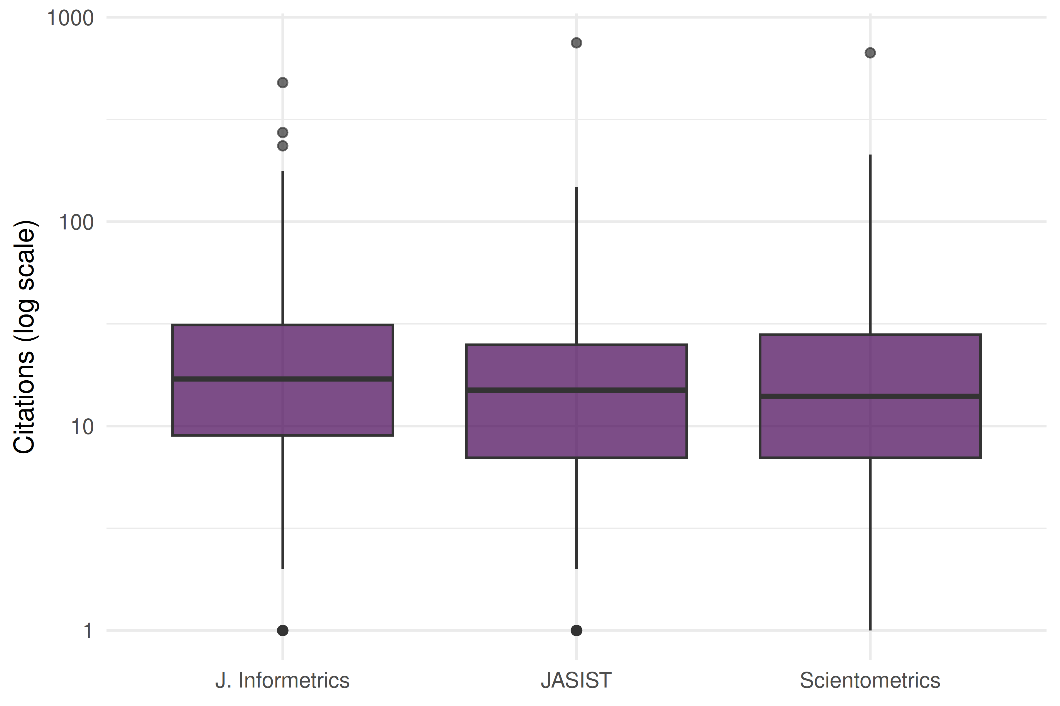

Figure 41.1: Citation count distributions by journal.

all_works |>
  group_by(journal) |>
  summarise(
    n = n(),
    mean_cites = round(mean(cited_by_count), 1),
    median_cites = median(cited_by_count),
    h_index = compute_h_index(cited_by_count),
    .groups = "drop"
  ) |>
  gt()

journal	n	mean_cites	median_cites	h_index
J. Informetrics	300	27.6	16	44
JASIST	300	21.5	14	38
Scientometrics	300	24.6	13	40

41.5 Citation aging

aging <- all_works |>
  mutate(age = 2024 - year(publication_date)) |>
  group_by(journal, age) |>
  summarise(mean_cites = mean(cited_by_count, na.rm = TRUE), .groups = "drop")

ggplot(aging, aes(x = age, y = mean_cites, colour = journal)) +
  geom_line(linewidth = 1) +
  geom_point(size = 2) +
  scale_colour_manual(values = palette_sci(3)) +
  labs(x = "Years since publication", y = "Mean citations", colour = "Journal") +
  theme_sci()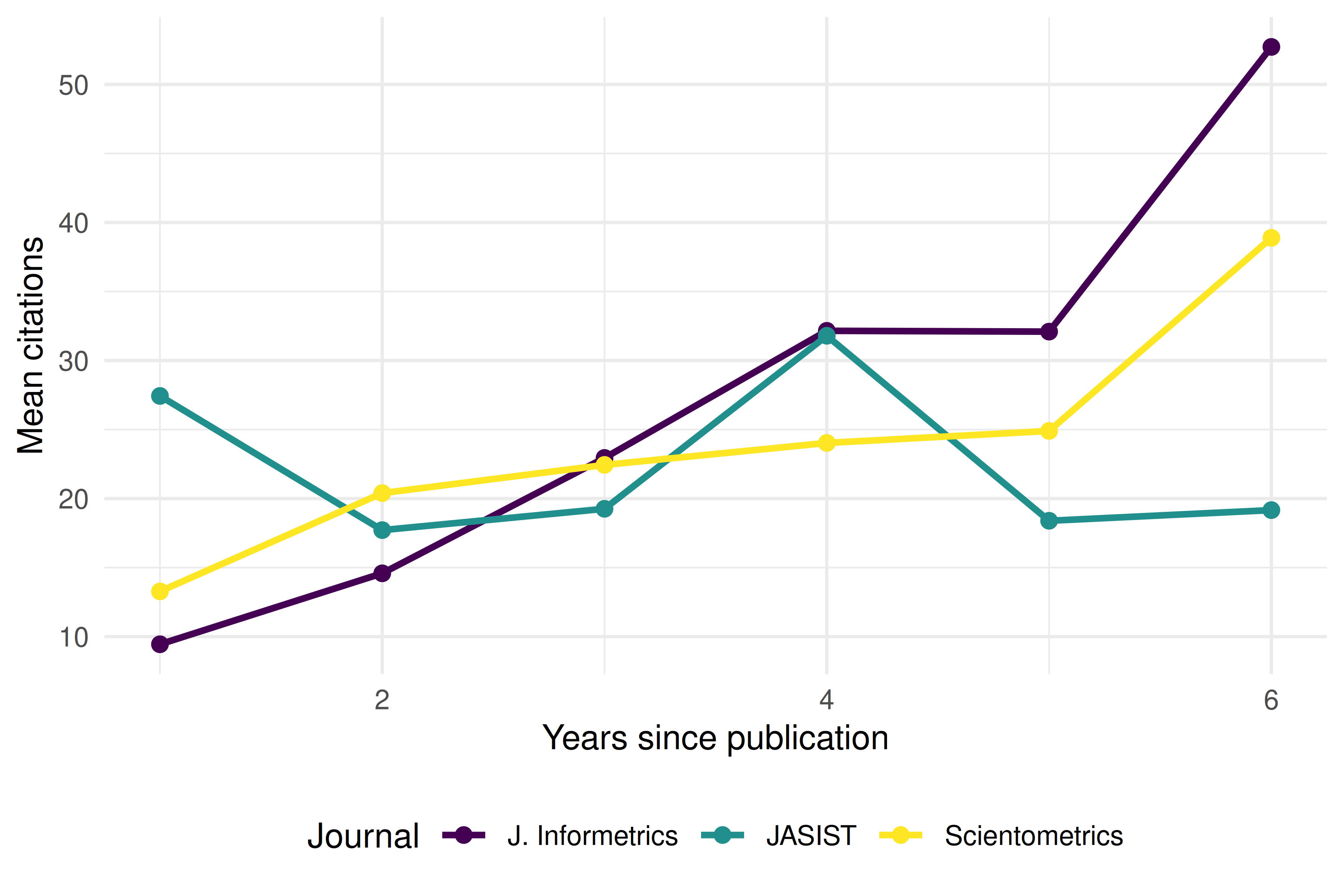

Figure 41.2: Mean citations by article age for each journal.

41.6 Topical coverage

topic_data <- all_works |>
  select(id, journal, topics) |>
  unnest(topics, names_sep = "_") |>
  select(journal, topic = topics_display_name) |>
  mutate(topic = str_to_lower(str_trim(topic))) |>
  filter(!is.na(topic), nchar(topic) >= 3)

top_topics <- topic_data |>
  count(journal, topic, sort = TRUE) |>
  group_by(journal) |>
  slice_max(n, n = 10) |>
  ungroup()

top_topics |>
  mutate(topic = reorder_within(topic, n, journal)) |>
  ggplot(aes(x = n, y = topic)) +
  geom_col(fill = palette_sci(1)) +
  facet_wrap(~ journal, scales = "free_y") +
  scale_y_reordered() +
  labs(x = "Frequency", y = NULL) +
  theme_sci(base_size = 9)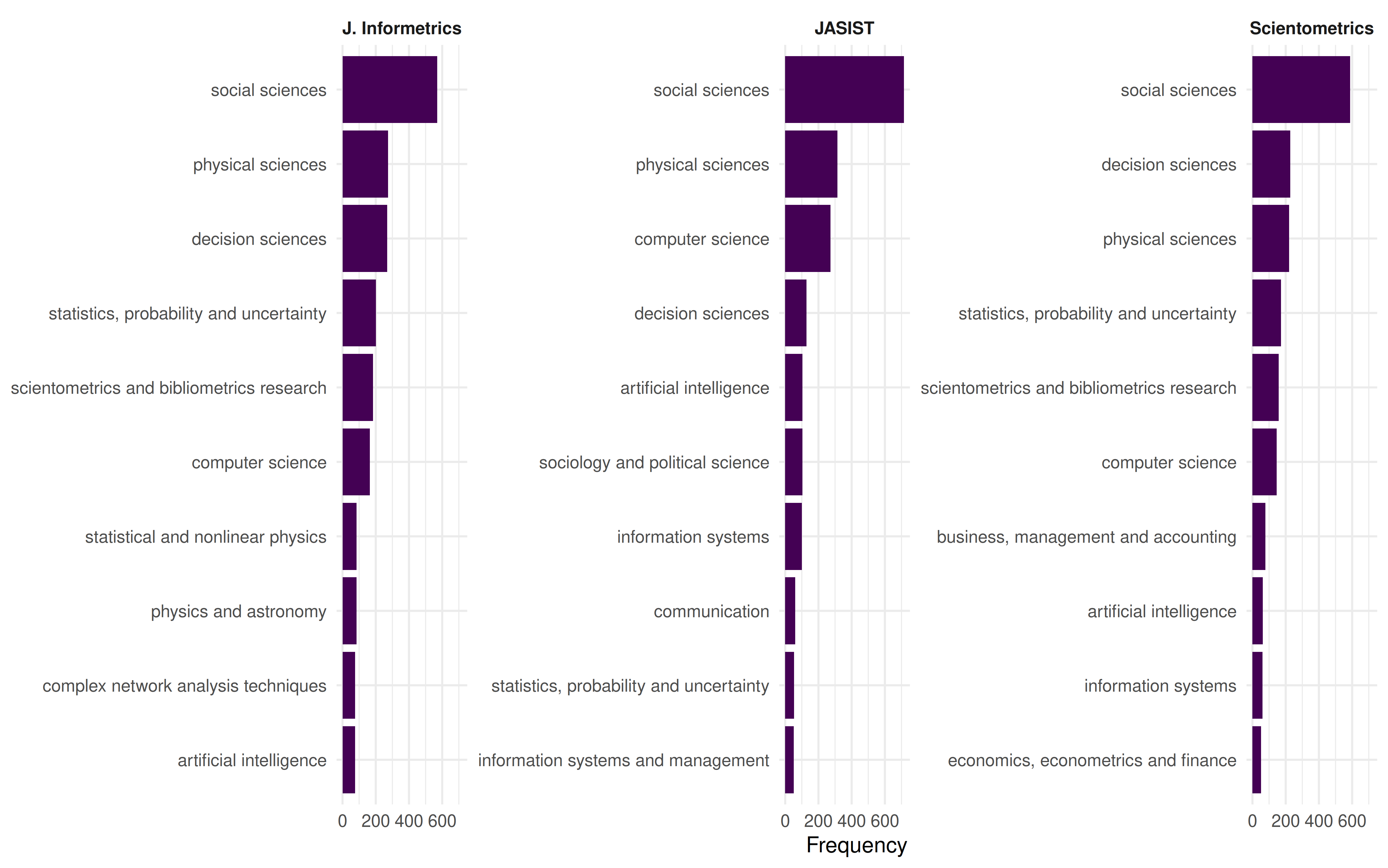

Figure 41.3: Top 10 topics by journal.

41.7 Key findings

1. Impact variation: Citation distributions differ across journals, with some showing higher medians and others higher means (driven by a few highly cited papers).
2. Aging patterns: All three journals show similar aging curves, consistent with the same broad discipline.
3. Topical differentiation: Despite overlapping coverage, each journal has distinct topical emphases.

41.8 Lessons learned

• Journal comparison requires multiple dimensions; no single metric tells the full story.
• Sample-based analysis is illustrative. For production-quality journal evaluation, use complete data and field-normalised indicators (Waltman 2016).
• Citation aging patterns are remarkably consistent within a discipline but would differ dramatically between, say, biomedicine and humanities.

This book was built by the bookdown R package.